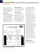
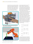
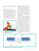
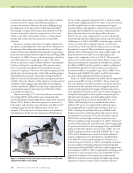
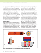
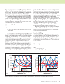
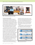
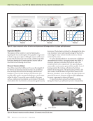
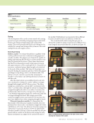
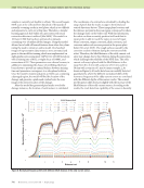
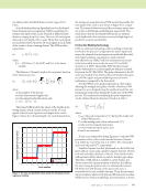
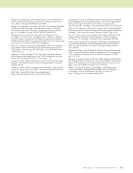
746 M A T E R I A L S E V A L U A T I O N • J U L Y 2 0 2 1 samples is currently not feasible to obtain. This would require NDE scans to be collected from hundreds of thousands of naturally occurring cracks in steel plates, which is too difficult and expensive to carry out at this time. Therefore, a transfer learning approach that builds off a preconstructed neural network architecture is utilized (Ma 2008). This model is a 101-layer CNN that has been pretrained on datasets containing over 15 million labeled images. Using this model allowed us to build off learned features from other data, elimi- nating the need to retrain an entire model. One hundred images of representative data instances were annotated and given to the model for training, which was implemented on eight graphics processing units (GPUs) for 160 000 iterations with a learning rate of 0.02, a weight decay of 0.0001, and momentum of 0.9. These parameters were chosen because, in addition to minimizing the chance of overfitting, they have been shown to provide an optimal balance between training time and premature convergence to a suboptimal solution. Once the model is trained and given an NDE scan containing a damaged region, the model will find the location of the damage and generate a pixel mask overlaid onto the scan image at the precise location of the damage. After the model has generated pixel masks over boiler damage instances, the location of each instance is calculated. The coordinates of a centroid are calculated by dividing the range of pixels that the masks occupy in horizontal and vertical directions by two. These image plane locations and the distance per pixel in the scan region correspond to where the damage exists on the boiler wall. With this information, the robot can then accurately position itself such that its repair probe is able to reach the region in need of repair. Steam corrosion, oxygen corrosion, alkali corrosion, and corrosion under scale are ever-present in the power plant boiler (Wu et al. 2019). The rough surfaces caused by the corrosion result in vibration during the movement of the robot. Therefore, the liftoff distance of the eddy current coil array may change due to this vibration during the inspection, which challenges the reliability of the NDE data. The eddy current coil array is placed with the liftoff distance in the range from 0 to 5 mm with a step size of 0.1 mm and 6 to 50 mm with a step size of 1 mm to inspect sample 2. As shown in Figure 8, all cracks have been successfully detected quantitatively, where the different normalized shifts of the resonance frequency of the eddy current sensor are correlated with the different depths of the narrow cracks. The normal- ized frequency shift decreases slightly with the increase of the liftoff distance of the eddy current sensor. According to the results, the crack detection capability of the sensor is basically ME TECHNICAL PAPER w ai-enabled robotic nde for structural damage 1 2 .1 .2 2 3 2 3 4 5 6 ( 7 8 9 10 11 1 2 3 4 5 6 7 8 9 11 12 13 14 15 16 1 18 19 20 21 22 23 24 25 L ( 26 2 28 29 30 31 32 33 34 35 6 37 38 40 41 2 44 45 47 8 9 0 2.4 2.5 2.6 Distance cm) 0 10 1 1 8 9 0 Liftoff distance (mm) 2 3 3 3 3 3 39 4 43 46 Figure 8. Normalized frequency shifts with different liftoff distance of the eddy current sensor. ×107 Normalized frequencyshifts

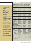
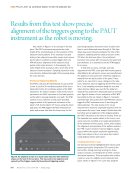
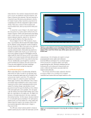
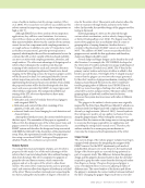
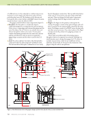
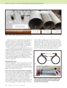
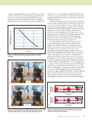
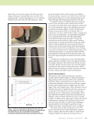
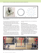
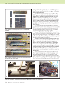
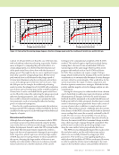
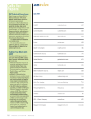
J U L Y 2 0 2 1 • M A T E R I A L S E V A L U A T I O N 747 not influenced by the liftoff distance in the range of 0 to 5 mm. A crack-depth prediction algorithm based on the kernel- based Gaussian process regression (GPR) is performed to estimate the depth of the cracks obtained at different liftoff distances ranging from 0 to 5 mm. There are 50 crack signals obtained at each depth of the cracks. Thirty-five crack signals are randomly selected from the 50 crack signals in each depth of the cracks to form a training dataset. The GPR model is expressed as: (1) where l(x) ~ GP(0,k[x,x´]), b(x) Rp, and l(xi) is the latent variable. The Matern 5/2 kernel is used as the covariance function of the Gaussian process: (2) where i is the number of the dataset, sl is the characteristic length scale, sf is the signal standard deviation, and r = √(xi – xj)T(xi – xj). The trained GPR predicts the values of the depths in the testing dataset, which consists of the rest of the 15 crack signals of the 50 crack signals in each depth of the cracks. Figure 9 shows the estimated depth of a crack obtained from the testing sets using the trained GPR model. Meanwhile, the true depth of the crack is also shown in Figure 9 for compar- ison. The mean absolute error and the root mean square error are as low as 0.0018 mm and 0.002 mm, respectively. The result shows that the developed GPR model can estimate crack depth with a low estimation error and a high degree of prediction accuracy and stability. Friction Stir Welding Technology FSW is a solid-state technology with no melting of materials involved in the process. Compared to the fusion repair tech- nique, the relatively low heat input associated with this solid- state repair technique can generate a much narrower heat-affected zone (HAZ) with less sensitization and a rela- tively low residual stress in the stir zone (SZ) and HAZ (Lienert et al. 2003). Meanwhile, FSW introduces large plastic deformation to activate significant dynamic recrystal- lization in the SZ (Ma 2008). The grain refinement in the SZ and a low residual stress lead to enhanced mechanical proper- ties of FSW repairs and potentially improved corrosion performance compared to the base metal. For the FSW process, peak temperature is a key output affecting the strength and quality of welds. Therefore, FSW parameters were designed using the analytical model for esti- mating peak temperature during the steady state of the FSW process. The equation for estimating the peak temperature can be obtained from the literature (Gosh et al. 2011): (3) where Tpeak is the peak temperature (°C) during the steady state of the FSW process, Tm is the melting point of low carbon steel (°C), v is the tool travel speed (mm/min), w is tool rotational speed (rpm), and K and a are constants. K and a are estimated by fitting Equation 3 with the FSW parameters of low carbon steel from the literature (Lienert et al. 2003 De et al. 2014 Cui et al. 2007). The estimated K and a are 0.82 and 0.177, respectively. Simulated repairs were first performed on a flat A108 steel plate without cracks using a pinless tungsten-rhenium (W-Re) tool with a shoulder diameter of 10 mm. Note that the boiler wall material is A106, which can only be found in pipe shape. Therefore, A108, which is available in a plate format, was chosen instead for repair parameter evaluation. In addition, the aim of using the pinless tool is to eliminate the keyhole left by the tool with the pin on the base metal, since a retractable tool is not available this time. Then, the prototype repair condition, which is 500 rpm and 80 mm/min, was iden- tified based on surface morphology characterization, as shown k x i ,x j ( ( ) = ’2 f + 5r ’ l + 5r2 3’l2 & % $1 # " ! exp 5r ’ l & % $ # " ! y l x) b(x) T ( = ¡ + Tpeak T m = K ( ’2 v (104 & % $ # " ! 5 10 15 20 25 30 35 40 45 0 3.8 4 4.2 4.4 4.6 4.8 5 5.2 Crack number True depth Estimated depth Figure 9. The true and predicted values using the Gaussian process regression method. Estimated depth of crack (mm)