where ​
ε​ is the dielectric constant, ​
μ​ is the magnetic permeability, and ​
σ​ is the electrical conductivity.
All of these provide the theoretical basis for the parame-
ter settings in the simulation software and facilitate the sub-
sequent validation of the correlation studies between the
data and the signal graphic accuracy, edge angle, and signal
changes.
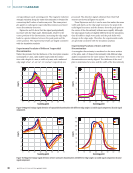
Also, when examining the effect of the edge angle of a dis-
continuity on the magnetic leakage signal, it is important to
recognize that the term “magnetic leakage signal” represents
the magnetic induction strength collected at the discontinuity
by the Hall element, reflecting the presence and location of the
discontinuity. The magnetic field strength, in turn, is usually
characterized by the magnetic induction strength, while the
variation and distribution of the magnetic field are described
by the gradient and curvature. From a physical perspective, the
gradient reflects the speed and direction of change in magnetic
field strength in space, serving as the maximum derivative of
a multivariate function in a specific direction, represented as
a direction vector. Curvature, on the other hand, is used in
mathematics to measure the degree of curvature of curves or
surfaces. In the magnetic environment, it describes the curva-
ture of magnetic field lines in space for example, the curvature
of the magnetic field lines around the edges of a magnet is
large, while the curvature in a region of uniform magnetic field
strength is small. The rate of change and degree of curvature
of the magnetic field strength are reflected by the gradient and
curvature, which in turn reveal the image characteristics of
the discontinuity’s presence (Long et al. 2021 ZhongCai et al.
2015). In other words, the edge angle, as a characteristic of the
discontinuity, affects the magnetic field gradient and curvature,
which change with the edge angle, ultimately influencing the
magnetic field strength and the acquired signal curve.
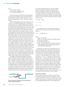
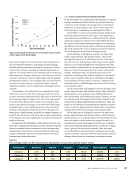
According to the principle that magnetic refraction is
similar to light refraction, the propagation and refraction of
magnetic field lines in different media (at the discontinuity)
behave similarly to the refraction of light waves. As shown in
Figure 1, consider a right-angled trapezoidal discontinuity with
an edge angle of 63° as an example. When transitioning from
one magnetic medium to another, the magnetic field lines at
the interface will suddenly change. Magnetic field lines are uni-
formly distributed within the same medium, but when travel-
ing through two media, a discontinuity occurs at the interface,
resulting in refraction. When magnetic field lines transition
from a high-permeability medium to a low-permeability
medium at the interface, they bend toward the normal
(Kim 2012 Assylbekov and Yang 2015). This indicates that
the magnetic field lines are horizontal within the ferromag-
netic sample and become perpendicular to the surface of the
sample when they enter the air. Therefore, the refraction angle
equation can be derived from the magnetic field line schematic
shown in Figure 1: ​ ​
(6)​ ​ n1​​sinθ ​ =​ n​2​​sin​θ2​​​​ ​ ​
(7)​ n =​ √
_εμ​​ ​ ​
(8)​ ​ θ​1​​ =​ π
2 ​
− α​
The relationship between the magnetic field refraction
angle and the edge angle can be derived from the following
equation: ​ ​
(9)​ ​ θ​2​​ =arcsin​
(​​
n1​​ ​ ​
n2​​​ ​ sin[​π ​
2 ​
− α])​​​
where
Equation 6 is Snell’s law, ​ ​
n​1​​​ and ​​ ​ 2​​​ are the refractive indices of two different media, ​ ​
θ​1​​​ is the angle of incidence, ​ ​
θ​2​​​ is the angle of refraction and
Equation 7 is the expression for the refractive index, where ​
ε​ is the permittivity and ​ ​ is the permeability, which is
affected by the DC magnetization.
Equations 8 and 9 express the relationship between the
magnetic field line incidence angle and the edge angle, and
the magnetic field line refraction angle and the edge angle,
respectively. Here, ​ ​ represents the angle between the direc-
tion of the magnetic field line and the boundary of the dis-
continuity, i.e., the edge angle, as shown in Figure 1. When ​ ​
varies from 0° to 90°, (​ ​ –​ α​ decreases as ​ ​ increases, and
similarly sin(​ ​ – ​ ​ becomes smaller. Therefore, according to
Equation 9, the refraction angle ​​ ​ 2​​​ also decreases. The change
in the direction of the magnetic field lines depicted in Figure 1
suggests that as ​​ ​ 2​​​ decreases, the curvature of the magnetic
field lines increases, potentially resulting in denser magnetic
field lines nearby. This indicates an increase in magnetic field
strength in the region and an increase in the strength of the
collected signal. Additionally, if the curvature of the magnetic
field lines changes, the location of the peak point of the
magnetic leakage signal will also shift. To confirm this, we will
use simulations and experiments for further validation.
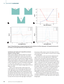
Finite Element Model
Leakage magnetic detection technology is a relatively static
low-frequency magnetization process, classified as a “static
magnetic field” problem. In this paper, COMSOL finite element
software is used to build a two-dimensional simulation model
for discontinuity leakage detection, to study changes in the
ME
|
MAGNETICLEAKAGE
Air
Magnetic field lines θ
1
θ
2
n
1
n
2 α
Figure 1. Schematic of magnetic refraction at the interface of a
trapezoidal shaped discontinuity.
32
M AT E R I A L S E V A L U AT I O N • M AY 2 0 2 5

axial and radial magnetic leakage field, and to obtain the rela-
tionship between the edge angle of discontinuities of differ-
ent shapes and the changes in magnetic leakage signals. To
simplify the calculation, a steel plate is used as the test sample,
with artificial defects machined on its surface to simulate real
conditions, as shown in Figure 2. The model includes a mild
steel sample, an excitation coil, a soft iron yoke, a Hall element,
and an artificial defect. The material properties of each part are
listed in Table 1.
In particular, when grid dissection is performed using
COMSOL software, focused calculations and grid encryption
are applied near the surface on the defect side to improve
the smoothness and accuracy of the leakage field acquisition
results.
Magnetic Leakage Signal Analysis of Discontinuities
with Different Edge Angles
In engineering, the edge angles of discontinuities can vary
arbitrarily between 0° and 180°. This paper focuses on the
study of discontinuity edge angles in the range of 0° to 90°, as
these angles are more common in actual working conditions.
Based on the principle of magnetic leakage detection and
COMSOL simulation, this paper presents several discontinuity
models and further investigates the characteristic relationship
between the edge angles of these discontinuity models and the
magnetic leakage signal.
Selection of Liftoff Values in Leakage Detection
The choice of liftoff value is one of the key factors affecting
the acquisition of a magnetic leakage signal. A suitable liftoff
value should be selected based on the actual detection of the
component. If the liftoff value is too small, friction may occur
with the sensor during the moving detection process, thus
shortening the service life of the sensor. Similarly, if the liftoff
value is too large, the signal collected by the sensor will be
weak and the sensor may not be sensitive to magnetic leakage
signals. Therefore, a right-angled trapezoidal discontinuity with
an edge angle of 63° is taken as the object of study, with liftoff
values of 0.2 mm, 0.5 mm, 0.7 mm, and 1 mm set. The results
of the simulated signals are shown in Figure 3.
From Figures 3a and 3b, it can be seen that the intensity
of the magnetic leakage signal decreases as the liftoff value
increases. The radial and axial magnetic leakage signals are
strongest when the liftoff value is 0.2 mm. Practical consid-
erations for the experimental process suggest using a higher
liftoff value to better protect the sensors from damage (Sun
and Kang 2010). This paper chooses a liftoff value of 0.5 mm
for the subsequent study.
Artificial
defect
Hall element
Soft iron yoke
Excitation coil
Low-carbon steel
Figure 2. Leakage detection simulation model.
TA B L E 1
Material properties of the components
Part Material Relative
permeability
Conductivity
(S/m)
Sample Carbon steel 400 8.41 ​ ​ 107
Excitation coil Copper 1 5.99 ​ 107
Yoke Soft iron 4000 1.12 ​ 107
80
70
60
50
40
40
50
60
70
80
90
100
110
120
30
30
20
10
–10
–20
–30
–40
–50
–60
–70
–80
–90
–100
0
0 5 10
Scanning path (mm) Scanning path (mm)
15 20 0 5 10 15 20
0.2 mm
0.5 mm
0.7 mm
1 mm
0.2 mm
0.5 mm
0.7 mm
1 mm
Figure 3. Distribution of radial and axial signals of magnetic leakage for different liftoff values: (a) radial signal component (b) axial signal
component.
M AY 2 0 2 5 • M AT E R I A L S E V A L U AT I O N 33
B
(mT)
B
(mT)