distributed at the discontinuity boundary, which increases the
magnetic field strength in this region and ultimately enhances
the amplitude of the collected magnetic leakage signal.
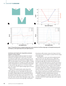
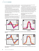
To illustrate the transition of the axial signal from a single
to a double crest, we take a right-angled trapezoidal discon-
tinuity with an edge angle of 63° as an example, keeping the
other parameters unchanged. By varying the width of the dis-
continuity and the magnitude of the magnetizing current, we
obtain the graphs shown in Figures 5e and 5f. A comparative
study of Figures 5e and 5d reveals that the effects of varying
the discontinuity width and the discontinuity edge angle on
the axial signals are similar, both leading to a change in the
number of wave crests.
The specific reason is that an increase in the discontinuity
width leads to a significant increase in the dispersion of the
magnetic field lines at the discontinuity edge (Li et al. 2017).
When the magnetic field lines pass through discontinuities
with larger widths, there is a significant scattering effect at the
discontinuity edges, leading to increased bending and reflec-
tion of the magnetic field lines, which generates multiple wave
peaks in the magnetic leakage signal. On the other hand, as
the edge angle of the discontinuity increases, the distribution
of the magnetic field lines on both sides of the discontinu-
ity changes (Feng et al. 2022), and a stronger magnetic field
gradient is generated in the discontinuity region. When the
magnetic field gradient is concentrated in a certain region,
the detection signal will show a single peak characteristic. In
the center region of the discontinuity, the signal strength is
weakened due to the highly dispersed magnetic field lines,
resulting in a divergent distribution. This change in distribu-
tion pattern eventually leads to a shift in the axial signal from a
single to a double peak.
By analyzing the changes in radial and axial signals, the
morphological dimensions of the discontinuity and the size of
its edge angle can be evaluated.
Simulation and Analysis of Magnetic Leakage Signal for
Inner and Outer Discontinuities
All of the above studies have explored the relationship between
the edge angle of unilateral discontinuities and the variation
of the magnetic leakage signal. However, the effect of edge
angle changes on the magnetic leakage signal on both sides of
the inside and outside of the sample still needs to be further
investigated.
ME
|
MAGNETICLEAKAGE
60
70
80
40
30
20
50
10
–20
–30
–10
–40
–50
–60
–70
–80
0
0 5 10
Scanning path (mm)
15 20
60
70
80
90
100
110
120
130
140
40
50
0 5 10
Scanning path (mm)
60
65
70
75
80
8.15
8.10
8.05
8.00
7.95
7.90
55
45° 63° 34°
Edge angle (degrees)
15 20
63°
45°
34°
63°
45°
34°
63° 45° 34°
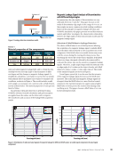
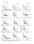
Figure 6. Inner and outer discontinuities and their magnetic leakage signal distributions: (a) model of the inner and outer discontinuities
(b) trend plot (c) radial signal component (d) axial signal component.
36
M AT E R I A L S E V A L U AT I O N • M AY 2 0 2 5
B
(mT)
B
(mT)
B
(mT)
L
t on
po
i

According to the principle of magnetic leakage signal
superposition, the theory should be consistent with the con-
clusion of the previous studies however, to improve the
accuracy of the conclusions, experimental simulation is carried
out again. Assuming that the thickness of the sample remains
unchanged at 5 mm, a rectangular discontinuity with a width
of 4 mm and a depth of 2 mm is set up on one side of the
sample, and a V-shaped discontinuity with a width of 4 mm
and a depth of 2 mm is set up on the other side. The edge
angles are set to 34°, 45°, and 63°, as shown in Figure 6a.
Figure 6c shows considerable fluctuations in the peaks on
both the left and right sides of the radial signal map. The radial
signal peaks increase with the edge angle and gradually move
away from the center position of the discontinuity. In Figure 6d,
the position of the axial signal peak gradually shifts to the left as
the edge angle increases, while the peak intensity also increases.
This is consistent with the trend plot in Figure 6b.
This finding supports the previous observation, demon-
strating that as the edge angle of the discontinuity increases, the
magnetic field lines on the discontinuity side become more con-
centrated. This concentration effect produces a strong magnetic
field gradient on one side of the discontinuity, which results in
the formation of distinct wave peaks in the detection signal.
Experimental Validation and Analysis
To verify the correctness of the simulation conclusions, we
built a simple magnetic leakage detection platform for the
experiment. The main equipment of the platform includes an
excitation coil, mobile platform, a Hall sensor, a microcontrol-
ler, a 5A AC/DC power supply, an experimental steel plate, and
a computer. The specific physical setup is shown in Figure 7.
During the experiment, the magnetic yoke and sensor are
driven horizontally by the moving platform at a constant speed
to collect point-to-point signals for the discontinuities on the
steel plate and present the data in the form of 2D curves on
the computer. This is consistent with the principle of COMSOL
simulation.
Experimental Analysis of Different V-shaped
Discontinuities
Discontinuities with depths of 0.73 mm, 2 mm, and 4.3 mm
were processed on a steel plate with a thickness of 5 mm.
V-shaped discontinuities with edge angles of 20°, 45°, and 65°
were created while keeping the discontinuity width constant
at 4 mm. The detection signals were obtained using Hall
sensors, as shown in Figures 8a and 8b. The X-axis represents
the number of scanning points along the discontinuities, while
the Y-axis represents the magnetic induction strength (B)
0 10
0
20
40
60
80
100
120
140
160
180
20 30
Scanning point
100
50
0
–50
–100
–150
150
40 50 60 70
0 10 20 30
Scanning point
40 50 60 70
65°
45°
20°
65°
45°
20°
Figure 8. Magnetic leakage signal detection of V-shaped discontinuities
with different edge angles: (a) radial signal component (b) axial signal
component.
Figure 7. Experimental test platform: (a) excitation coil (b) mobile
platform (c) Hall sensor (d) microcontroller (e) steel plate.
M AY 2 0 2 5 • M AT E R I A L S E V A L U AT I O N 37
B
(mT)
B
(mT)