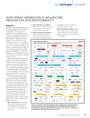
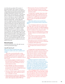
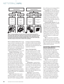
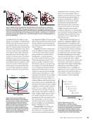
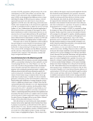
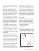
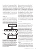
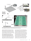
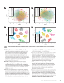
NDT/E, obtaining reliable labels is a spe- cialized and time-consuming task, which is further complicated as manual delin- eation of discontinuities introduces user subjectivity. In turn, mislabeled data can be counteractive to the learning process of supervised learning ML models (Taheri and Zafar 2023 Lever et al. 2017). Unsupervised learning: An ML paradigm from which an ML model is trained from the input data features, but without known data labels. Clustering is one of the most well-known forms of unsupervised learning, wherein data is divided into discrete groups. Furthermore, dimensionality reduc- tion and manifold learning methods such as principal component analysis (PCA) (Lever et al. 2017 Yang et al. 2022) and t-distributed stochastic neighbor embedding (tSNE) (van der Maaten and Hinton 2008) are forms of unsuper- vised learning. Unsupervised learning is useful in NDT/E due to the challenges of obtaining labels. Tips: If dependable labels can be obtained for a dataset, a supervised learning paradigm is often the simplest and most accurate. Assuming no labels are known, unsupervised learning is powerful but requires domain-specific insights from the user. Unsupervised learning also generally lacks metrics for standardized evaluation. Types of Learning Tasks Each ML paradigm can take on differ- ent tasks. In this subsection, we sub- divide supervised learning into its two most common tasks (classification and regression) and subdivide unsupervised learning into its two most common tasks (clustering and dimensionality reduc- tion). These subgroups are illustrated in Figure 1. Classification: A supervised ML model performs classification when it determines if the input data belongs to one of a discrete set of “classes,” or cat- egories. For example, different defect types (e.g., delamination, crack, no defect) may represent different classes that we may observe. Regression: A supervised ML machine model performs regression when estimating the value of a contin- uous dependent variable from an input independent variable. For example, an ML model may process imaging NDT/E data to estimate the size of a defect. Clustering: The clustering task aims to classify data without known informa- tion by identifying groups, or clusters, of data that are similar to each other in some manner. Clustering can be valuable for identifying unknown rela- tionships between the data, such as the presence of outlier data that could corre- spond to a discontinuity. Dimensionality reduction: The aim of dimensionality reduction is to reduce the data into its essential features. Many compression and denoising algorithms can be considered forms of dimensionality reduction (Yang et al. 2022). It can separate components (e.g., multiple reflections from an ultrasonic B-scan) that reconstruct the data when added together (Liu et al. 2015). This is sometimes referred to as blind source separation. Tips: It is important to determine the appropriate learning task for a given problem as it dictates the choice of an ML model and the associated challenges. Figure 1 describes the most common ML models used for each task. Characteristics of Machine Learning Datasets and Architectures Most ML architectures learn only from the provided data. As a result, ML model performance is highly depen- dent on the dataset quality. The classic bias-variance tradeoff is one of the most common challenges we must consider when building a dataset and choosing an architecture. Bias: One of the most significant issues that one must consider when creating a dataset is to consider the inherent bias that the dataset exhibits and how it affects the ML model. That is, a dataset will be biased if the training data (i.e., the input data and labels that are used to initially train the model) tends to better represent one scenario over another (Mehrabi et al. 2022). Note that bias is not inherently bad since you may want to focus on a particu- lar scenario (Miceli et al. 2022), but it is important to acknowledge that bias. For example, an ML model trained NDT TUTORIAL |AI/ML Labeled data Supervised learning Classification Regression Support vector machine Decision trees Random forests Linear regression Regularized regression Support vector regression Unlabeled data Unsupervised learning Clustering Dimensionality reduction K-means clustering Density-based clustering Principal component analysis Non-negative matrix factorization Figure 1. Learning paradigms of machine learning: (a) supervised learning algorithms utilize labeled data, which allows algorithms to be trained directly on the downstream task (classification and regression) (b) unsupervised algorithms utilize unlabeled data, which are primarily used for clustering and dimensionality reduction. Semi-supervised learning algorithms incorporate characteristics of both of these paradigms. 44 M A T E R I A L S E V A L U A T I O N • J U L Y 2 0 2 3 2307 ME July dup.indd 44 6/19/23 3:41 PM

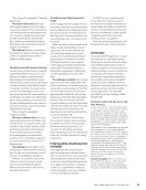
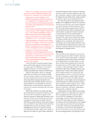
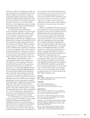
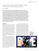
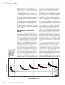
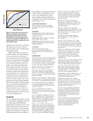
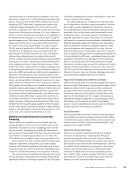
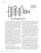
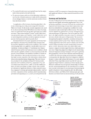
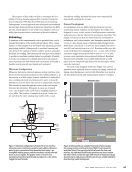
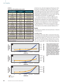
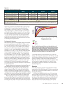
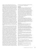
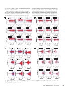
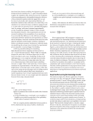
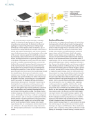
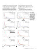
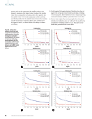
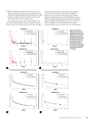
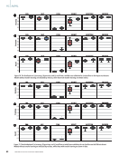
on simulated data (for which we can produce an abundance of labeled data) will learn the specific characteristics of the simulated data, but it may not also represent experimentally measured data. If the labels are imbalanced (e.g., there are twice as many cracks as delamina- tions), then the data will be inherently more likely to predict the larger class. In short, if a characteristic of our data is imbalanced (e.g., twice as many mea- surements originate from aircraft wings than bridges), then the predictions will be more accurate for those dominant characteristics. An underfit ML model is created when trained with a biased dataset or when the ML model has too few parameters (Figure 2). Such a model fails to learn specific characteristics from the data, leading to poor performance (the classic bias-variance tradeoff is illus- trated in Figure 3). Variance: The effects of data imbal- ances are difficult to gauge in part due to the variance in the dataset, another factor that must be considered when building data. A common question posed by non-ML practitioners is often “How much data do you need?” The answer is usually “it depends” due to the inherent variance in the input data. For example, if a crack looks identical in every single measurement, then the dataset has very low variance. In this scenario, you may not need a learning system because one datum of a crack sufficiently describes all other examples (although some pattern recognition is still necessary). In contrast, if there are a million different and unique permuta- tions of how a crack is represented, then the ML model will need at least a million examples to correctly classify cracks. In reality, there are usually complex rela- tionships between all data correspond- ing to cracks, which the ML model can learn. A highly variable dataset with too few training examples and too many parameters to learn can yield an overfit ML model (Figure 2). Such a model may find uninformative relationships in noise, leading to poor performance (Figure 3) (Belkin et al. 2019). Interpretability: One should also consider the interpretability of an ML architecture. An interpretable ML model is one from which humans can comprehend how a decision is made (Du et al. 2019). In general, there is a negative correlation between accuracy and model interpretability (Figure 4). Gaining interpretability is a difficult problem due to the nature of black- box models, non-linearities, and high-dimensional data visualizations. Deep neural networks are the prime example, being the most accurate models but with little to no interpretabil- ity of the model decision-making. On the other hand, linear models (e.g., linear regression) are very interpretable, yet often less accurate. Tips: Misunderstanding bias and variance is a significant pitfall for early ML practitioners. For example, novice deep learning practitioners often default toward increasing the number of layers in a neural network, thereby increasing the model complexity. However, such an architecture is not only more compu- tationally demanding but can in some cases be less effective (due to overfitting) and less interpretable than a simpler architecture. For this reason, deep neural networks are unfavorable in situations with limited data samples of potentially high variance and situations where interpretability and accountability are important. In such a scenario, users may often analyze their problem using con- ventional ML models, such as support vector machines or linear regression Figure 2. Model fitting: (a) underfitting (b) ideal fitting and (c) overfitting. An underfitting model characteristically suffers from poor performance in the training data, being unable to learn the relationships within the data. On the other hand, an overfitting model characteristically suffers from over-performing on the training data (often viewed as “memorization”) and fails to generalize onto new data samples. Thus, a fundamental goal of machine learning algorithms is to find an ideal fitting. High bias Low variance Underfitting Low bias High variance Overfitting Optimal Variance Generalization error Bias2 Model complexity Figure 3. Bias-variance tradeoff curve. Machine learning models strive to balance bias and variance. Simple machine learning models typically have fewer parameters, wherein the high bias and low variance are characteristic of model underfitting. On the other hand, complex machine learning models have a large number of parameters, wherein the low bias and high variance are characteristic of model overfitting. Deep neural networks High High Low Random forests Support vector machines K-nearest-neighbors Decision trees Linear regression Interpretability Figure 4. Model accuracy versus interpretability. In machine learning, increased accuracy has a natural consequence of decreased interpretability. Accurate models tend to capture nonlinear and non-smooth relationships, while interpretable models tend to capture linear and smooth relationships. J U L Y 2 0 2 3 • M A T E R I A L S E V A L U A T I O N 45 2307 ME July dup.indd 45 6/19/23 3:41 PM Prediction error Accuracy