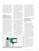
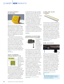
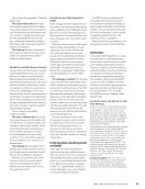
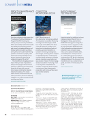
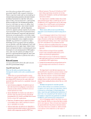
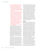
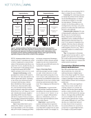
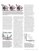
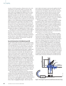
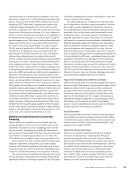
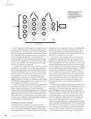
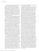
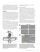
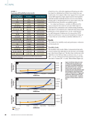
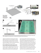
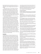
In NNs, weights are coefficients that act as scaling factors for the output of any given layer in an NN. They are the fundamen- tal parameters of an NN, and the aim is to optimize the values of these scalars to minimize the objective (or loss) function during the training phase. Back propagation (also known as backprop for short) is the primary algorithm for performing gradient descent on NNs. It involves performing a forward pass through the network by computing the output value of each node. Then, a backward pass through the network is performed, adjusting the values of the weights in the network. A weighted linear combination of all its inputs is calculated at each neuron. The inputs to the neurons are multiplied by their corresponding weights and then summed up. The result is then passed through an activation function. The activation function decides if the neuron should be activated or not and, if activated, decides its value. The sigmoid function is one example of an activation function. Training an NN requires defining the objective or loss function, typically the mean squared error (MSE) for regression problems or the cross-entropy loss for binary classification problems (relevant to NDT). With the rise of more powerful hardware, especially graphics processing units (GPUs), NNs can now be trained faster, requir- ing less computational hours while simultaneously being “deeper.” The “deep” in deep learning simply refers to the depth of layers in an NN, typically in the hundreds and thousands of hidden layers. The use of deep NNs has revolutionized the field of AI and ML, and frameworks such as PyTorch allow engineers in various fields to apply these powerful algorithms to problems in their respective domains of expertise. CONVOLUTIONAL NEURAL NETWORK CNNs, also known as ConvNets, are a class of NNs that are exceptionally well-suited for applications involving images and videos, such as image and video recognition, driverless cars, and image classification. Like ANNs, CNNs have an input layer, hidden layers, and an output layer. However, the hidden layers will have one or more convolution layers (hence the name). In conjunction with the convolution layers, CNNs also have pooling layers, and together form a single layer of a CNN. The architecture of a CNN is shown in Figure 3. The function of the convolution layer is to detect specific features in an image using the convolution operation that utilizes the concept of the inner (or dot) product between two vectors. In a CNN, the convolution operation is executed using a kernel that is the same size as the window of data it operates on. It is important to note that the kernel elements are weights the network learns when trained. The pooling layer is utilized to reduce the spatial dimension of the data, which helps reduce computational costs and makes the network resistant to overfitting. Each convolution layer has a rectified linear unit (ReLU) activation function that converts all negative values to zeros. The fully connected layer is not a characteristic of the CNN and contains an activation function just like an ANN, converting features into class probabilities (in classification problems). CNNs can process data with a similar grid structure. Local connections, weight sharing, and down-sampling are the main characteristics of CNNs that make them suitable for several types of AE signal analysis. CNN methods are based on the translation invariance of feature extraction and ignore the time correlation of signals. In the case of cyclic NNs, the complex structure and numerous parameters involved in the process make them difficult to optimize and train. Considering these limitations and challenges, research needs to be done to enhance the application of deep learning techniques for AE in situ monitoring for manufacturing processes, specifically in the case of AM. Li et al. (2022) presented a new AE signal recogni- tion method based on a temporal convolution network called acoustic emission temporal convolution network (AETCN) for real-time polymer flow state monitoring in an FDM process. ME |AI/ML Figure 2. An artificial neural network with various components labeled. The arrow shows the direction of back propagation. Weights Neurons Input size Back propagation Input layer Hidden layer 1 Hidden layer 2 Output layer Output size 54 M A T E R I A L S E V A L U A T I O N • J U L Y 2 0 2 3 2307 ME July dup.indd 54 6/19/23 3:41 PM

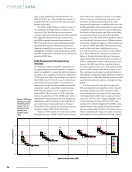
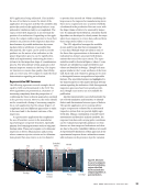
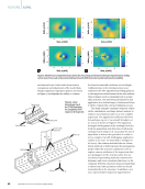
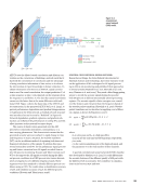
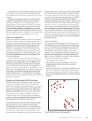
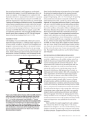
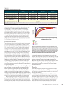
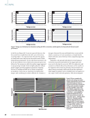
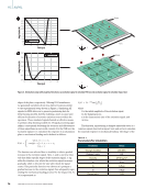
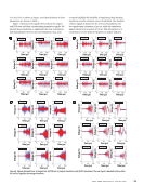
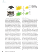
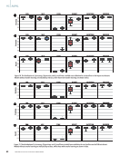
AETCN uses the dilated causal convolution and dilation con- volution as the cornerstone of building a network such that it has both the convenience of convolution and the advantage of using correlation information of time series, so it reduces the intervention of expert knowledge in feature extraction. To obtain information over time in an AETCN, causal convolu- tion is used. In causal convolution, the output prediction Yt of a time sequence at time t only depends on the timesteps from the sequence Xt and before Xt. The fact that causal convolution cannot see the future data is the main difference with tradi- tional CNN. Figure 4 shows the basic idea of the AETCN and its construction. In the proposed AETCN by Li et al. (2022), to prevent performance degradation and gradient disappearance or explosion in the deep network, a residual network structure was introduced as can be seen by “Resblock” in Figure 4b. Network degradation, gradient explosion, and gradient sub- traction can influence the performance of a deep NN, and this effect increases as the network becomes deeper. The source of elastic waves generated over the AM processes is commonly intermittent, nonstationary, or a time-varying phenomena. This characteristic means that the generated acoustic waves are subject to rapid change in time and frequency. In such a situation, the wavelet transform (WT) can be an efficient method of capturing both time and frequency information of the signals. To address this issue, several researchers used WT for the preliminary signal process- ing and feature extraction from AE signals recorded from in situ AM process monitoring. Hossain and Taheri (2021a) used WT to decompose the AE signals recorded during the differ- ent process conditions in a DED process into various discrete series of sequences over different frequency bands. These segments were then analyzed to identify different process con- ditions using a CNN. The results show a classification accuracy of 96% and validation accuracy of 95% for different process conditions (Hossain and Taheri 2021a, 2021b). SPECTRAL CONVOLUTIONAL NEURAL NETWORK Researchers at Empa, the Swiss Federal Laboratories for Materials Science and Technology, have done extensive work on the application of ML techniques for AE signal process- ing in AM in situ monitoring and published their approaches in several articles (Masinelli et al. 2021 Shevchik et al. 2018, 2019 Wasmer et al. 2018, 2019). They used a fiber Bragg grating sensor to record the acoustic signals during the powder bed AM process at different intentionally altered processing regimes. The acoustic signals’ relative energies were consid- ered the features and extracted from the frequency bands of the wavelet packet transform (Shevchik et al. 2018). Wavelet packet transform can be described as applying a set of filters on a signal, as shown by Equations 1 and 2: ​ ​ (1)​ ​ φ​j​​​(n)​ =​ ∑ n​ ​ ​ h0​​​(k)​√M​ ​ ​ _φ(Mn ​ − k)​, k ⊂ Z​​ ​ ​ ​ (2)​ ψ​ji​​​(n)​ =​ ∑ n​ ​ ​ hm−1​​​(k)​√M​ ​ ​ _ψ(Mn ​ − k)​, k ⊂ Z​​ where ​ ​ h​0​​​ is a low pass and ​​ ​ m​​​ is a high pass filter, φ and ψ are the scale and wavelet functions, respectively, j is a scale, n is the current sampling point of the digitized signal, and the parameter m is the total number of filter channels. A spectral convolutional neural network (SCNN) classifier was developed by Mathieu et al. (2014). It could differentiate the acoustic features of the different quality of AM parts with the different level of porosities. The confidence in classifica- tions varies between 83% and 89%. Conv-1 Conv-2 Conv-3 Conv-4 FC-6 FC-7 56 × 56 × 256 28 × 28 × 512 14 × 14 × 512 7 × 7 × 512 1 × 1 × 4096 1 × 1 × 1000 224 × 224 × 64 FC-8 Conv-5 Convolution +ReLU Max pooling Fully connected +ReLU 112 × 112 × 128 Figure 3. A convolutional neural network (CNN) model. J U L Y 2 0 2 3 • M A T E R I A L S E V A L U A T I O N 55 2307 ME July dup.indd 55 6/19/23 3:41 PM SOURCE: LEARNOPENCV (2023)