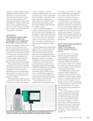
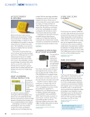
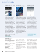
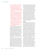
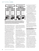
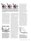
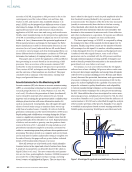
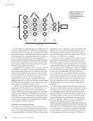
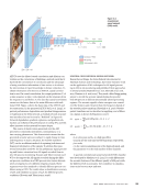
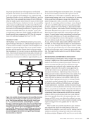
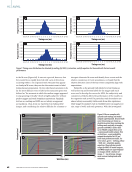
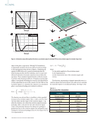
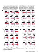
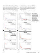
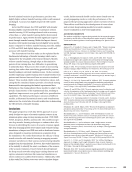
REINFORCEMENT LEARNING Using the same dataset, the Empa group studied the appli- cation of a reinforcement learning (RL) approach to classify different levels of quality for parts manufactured using AM (Wasmer et al. 2019). The RL technique is inspired by the human cognitive capabilities of learning in its surrounding world. In RL, knowledge is acquired through trial and error (or reward and penalty) in an environment by performing the actions and seeing the results of actions (Sutton and Barto 2018). In their approach, a Markovian process is the way of interaction between the RL agent and the environment. The initial state was set to ​​ ​ 0​​​ in the classification process and the algorithm reached the goal ​​ ​ g​​​ by the actions that win the maximum reward. The governing equation for the optimal reward is given by Equation 3: ​ ​ (3)​ ​​ ​​ ​​ ​​ ​ Tπ​​​(s)​ ​ =E​ {​ ∑ t​ ​ λR(​s​t​​, ​ π[​s​t​​]​)​​|​​​s​0​​ ​ =s​ }​ ​ where E is the expectation, the discount factor λ ⊂ [0,1), and π(st) is a policy that maps the states to the actions, and R is the space of the rewards. ME |AI/ML Padding unit Input layer Hidden layer Output layer Y t –2 d =8 d =4 d =2 d =1 Y t –1 Y t X t –2 X1 X2 X3 … … X t –1 X t Detail construction of Resblocks Previous Resblock Resblock Output Softmax Fully connected Resblock Resblock Resblock Input AE signals 9 Resblocks Skip connection 8 4 2 Dilation rate Drop out ReLU Weight norm Dilated causal convolution Drop out ReLU Weight norm Dilated causal convolution 1D convolution Next Resblock Figure 4. Acoustic emission temporal convolution network: (a) basic concept (b) construction (Li et al. 2022). 56 M A T E R I A L S E V A L U A T I O N • J U L Y 2 0 2 3 2307 ME July dup.indd 56 6/19/23 3:41 PM …

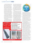
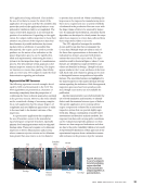
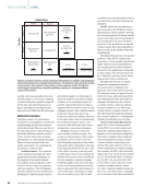
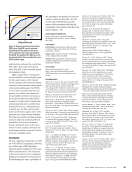
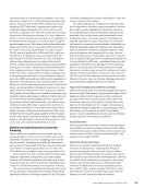
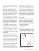
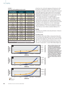
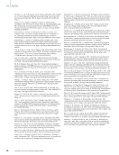
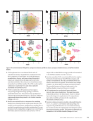
The confidence level of the RL-based classification in this case (Wasmer et al. 2018) was between 74% and 82%, which shows a slightly lower performance compared to their SCNN approach. Despite the encouraging results from the SCNN and RL, researchers at Empa empowered their acoustic-based ML approach by verifying the results using high-speed X-ray imaging techniques. Four categories of conduction welding, stable keyhole, unstable keyhole, and spatter were defined in a laser welding experiment and gradient boost with both independent component analysis and with CART were used to classify the different process conditions. 74% to 95% of accuracy was achieved in their assessments (Wasmer et al. 2018). SUPPORT VECTOR MACHINE Support vector machines (SVMs) can be used for both classi- fication and regression problems, although typically used for classification. The idea behind the SVM is to find the optimal hyperplane (the hyperplane with the highest margin) that separates the two classes. SVM is fundamentally a binary classifier, and a hyperplane is a decision boundary that sep- arates the two classes. If the dimension of the input data or the number of features is two, then the hyperplane is a line. For a three-dimensional feature space, the hyperplane is a two-dimensional plane. AE, in combination with accelerometers and thermo- couples data, was used by Nam et al. (2020) to train an SVM algorithm for diagnosing health states of the FDM process. The researchers first obtained the RMS values from the AE, accelerometers, and thermocouples data. They applied both linear and nonlinear SVM algorithms to identify the state of the FDM process as healthy or faulty. This research is a good case study of how to use SVMs for studying an AM process with the help of AE. However, it is to be noted that the SVM algo- rithm is ineffective when the dataset has more noise, which is a downside of using AET. Unsupervised Classification of AM Process States Unsupervised learning is a learning paradigm that does not require prior knowledge of the solution to the problem at hand, which implies that specifying the output is not required, or in some cases where such data may not be available. The implications of this approach are that we can learn inherent patterns in the data that we were not privy to there may be several solutions to the problem and different results can be obtained each time we run the model. In the following sections, we discuss the application of specific unsupervised learning algorithms to the study of AM using AET. CLUSTERING BY FAST SEARCH AND FIND OF DENSITY PEAKS The clustering by fast search and find of density peaks (CFSFDP) approach was used by Liu et al. (2018) to identify the FDM process state. Liu et al. used reduced feature space dimension by combining both time and frequency domain features and then reducing them with the linear discriminant analysis for their work. Consequently, CFSFDP, as an unsuper- vised density-based clustering method, is applied to classify and recognize different machine states of the extruder (Liu et al. 2018). Density-based clustering methods such as CFSFDP used by Liu et al. update the clusters iteratively without grouping the data. This approach is contrary to distance-based clustering methods such as hierarchical and partitioning algo- rithms like k-means. As a result of using CFSFDP, the FDM machine states were identified within a much smaller feature space, which helps to reduce the computational cost of classi- fication and state identification. Liu et al.’s work declared that reducing dimension in feature space remarkably improves the efficiency of state identification. For dimensionality reduction, the operator part of the algorithm can be customized by linear discriminant analysis. K-MEANS CLUSTERING The k-means clustering algorithm is one of the most widely used algorithms due to its flexibility and ease of implementa- tion. It is an unsupervised learning algorithm, a class of ML algorithms that can find patterns within a dataset without being explicitly told what the underlying mechanism is or might be. The only user-defined parameter required to train a k-means clustering algorithm is the number of clusters, k. Figure 5 shows an example of two clusters, with optimal loca- tions of centroids represented by triangles. The algorithm works as follows: 1. The user defines the number of clusters, k, and a corre- sponding number of cluster centroids (or means) are randomly chosen. 2. Each observation (or point) in the dataset is assigned to one of the clusters, based on its distance from a given centroid. There are several metrics used in ML to compute distances, but a commonly utilized measure is known as the Euclidean distance. Figure 5. Setup for a k-means clustering algorithm. J U L Y 2 0 2 3 • M A T E R I A L S E V A L U A T I O N 57 2307 ME July dup.indd 57 6/19/23 3:41 PM