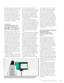
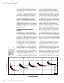
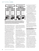
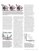
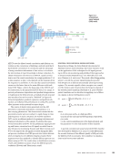
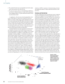
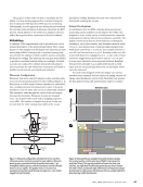
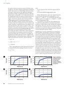
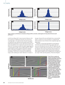
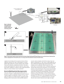
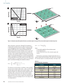
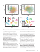
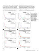
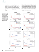
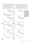
the regions of interest in ultrasonic scans and facilitate image cropping (see the Model Training and Performance Evaluation Section). The M-scans were labeled (Figure 2b) for the timing of four types of key events (see the cumulative distribution function plots in Figure 3): melting (the moment at which the molten nugget was first visible 17 102 events) steel-steel inter- face disappearance (SSID the moment at which all steel-steel interfaces appeared to have been breached by the molten nugget 16 907 events), saturation (the moment at which the molten nugget appeared to stop growing vertically 14 500 events) and expulsions (all first moments of discontinuity in the M-scan, which were suspected to be due to expulsion 6375 events). In addition, the top and bottom of the nugget as well as the top and bottom of the stack were labeled, relative to the ultrasonic M-scan, at the moment of saturation. As observed in the M-scan, historical vertical maximum nugget size (MNS) proportional to the stack throughout the weld was then derived from these labels. To derive MNS, a linear interpolation l between melting-event timestamp to saturation-event time- stamp (horizontally) and zero to maximum overall nugget size proportional to the stack (vertically) was first computed. Given melting timestamp m, saturation timestamp s, maximum overall size proportional to the stack n, and weld timestep t: ​nugget l =0, if t m​ ​ l =​ t − m _s − m ​ × n, if m ≤ t ≤ s​ ​ l =n, otherwise​ Then, a sigmoidal function of the following form was fitted to l using the SciPy software package (Virtanen et al. 2020): ​ y =​ n _1 +​ e​​ −a × ​ ​ ​ t−b​ ​​​​ ​ where a is a free parameter that controls the nugget growth rate, and b is a bias that shifts the nugget growth in time. Finally, a blend between l and y was computed such that the curve began fully linear at the melting point (i.e., the weight of l =1, weight of y =0) and ends fully sigmoidal at the saturation point (i.e., the weight of l =0, weight of y =1). MNS was the resultant blended curve. Consequently, at each time step of the welding process, the model was tasked with binary classification for the first occurrence of each of the key events: melting, SSID, saturation, and expulsion. That is, for each event, the model was tasked to output zero for every time step prior to the first occurrence of the event and one for every time step thereafter. The model was also tasked with regression of MNS. Model Design, Training, and Performance Evaluation The machine learning task defined previously is essentially many-to-many sequence processing. Many-to-many sequence processing produces any number of sequential outputs given any number of sequential inputs here, for every A-scan input the model is tasked with producing a corresponding output that describes the occurrence of events and MNS. All outputs are real numbers in the range of zero to one. A 1 ms per A-scan processing time constraint was imposed due to the required temporal resolution and response time such that feedback to a weld controller is actionable, as well as the rate of data acqui- sition such that the AI system does not accumulate latency throughout the course of a weld. Due to the severe computa- tional time constraint of 1 ms per A-scan, the aim to maximize performance, and the sequential nature of the ultrasonic data, a recurrent neural network approach was investigated. In par- ticular, to exploit the spatial information in each A-scan and ME |AI/ML Weld time (ms) Weld time (ms) Weld time (ms) Weld time (ms) 20 000 15 000 10 000 5000 0 0 100 200 300 400 20 000 15 000 10 000 5000 0 0 100 200 300 400 20 000 15 000 10 000 5000 0 0 100 200 300 400 20 000 15 000 10 000 5000 0 0 100 200 300 400 Figure 3. Cumulative distribution functions for the four events over the entire dataset: (a) melting (b) SSID (c) saturation (d) expulsion. 64 M A T E R I A L S E V A L U A T I O N • J U L Y 2 0 2 3 2307 ME July dup.indd 64 6/19/23 3:41 PM E count E count E count E count

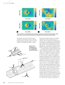
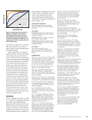
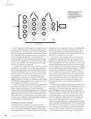
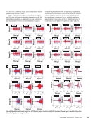
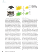
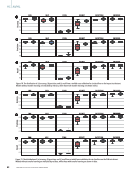
long-term dependencies in weld sequences, convolutional long short-term memory (ConvLSTM) architectures (Shi et al. 2015) were explored. All investigations were conducted with Tensorflow (Abadi et al. 2015) and Keras (Chollet et al. 2015) for Python. Due to the sequential processing of ConvLSTMs and relatively small sequence items (resized A-scans see the Model Training and Performance Evaluation Section), the amenability of processing to parallelization is heavily reduced for this task, and it was consequently found in preliminary work that CPUs were faster for both training and inference. Sequence process- ing using ConvLSTM differs from, for example, a pure CNN or transformer architecture, which is highly parallelizable and benefits greatly from computing on GPU. Thus, all computa- tions were performed using an Intel® Core™ i7 CPU. FEASIBILITY STUDY The feasibility of a ConvLSTM-based architecture was inves- tigated with input M-scans (i.e., arbitrary-length sequences of A-scans) resized vertically to 128 pixels. This investigation was designed to estimate the upper limit on the number of filters per layer and the number of layers based on the processing time requirement of 1 ms per A-scan in a production environ- ment, which includes input preprocessing and potential com- munications overhead. Preliminary tests determined that the production environment ran inference approximately 35–45% faster than the development environment due to, for example, the removal of training overhead in the exported network graph, differences in Tensorflow compilation, differences in programming language, and so on. Accounting for the speedup in the production environment, along with overhead from preprocessing and so forth, a cutoff of 1.1 ms per A-scan was imposed. An overarching architecture (Figure 4) was designed with one ConvLSTM module and one max pooling operation per layer variants were tested having 1–5 layers and an initial layer with 8–32 filters, with number of filters doubling per layer. Following a flattening, the last layer was a time-distributed (i.e., shared across all time steps) fully connected layer with five outputs. To guard against extra computational overhead from initial resource allocation, one M-scan was fully processed prior to recording inference times. Subsequently, 10 randomly selected, arbitrary-length M-scans, comprising of a total of 2589 A-scans, were processed, during which inference times were recorded. As M-scan length has no impact on mean inference time per A-scan, though it may subtly impact variance of infer- ence times, the selected M-scans were held constant through all trials so that the same exact A-scans were processed in each trial. The largest feasible model was used for further training and evaluation. MODEL TRAINING AND PERFORMANCE EVALUATION At both training and testing time, M-scan images were cropped vertically to tightly focus on the welded stackup, resized to a height of 128 pixels, and cropped horizontally starting at the current-on timing until the end of the weld process. Data augmentation was conducted only at training time and was designed to desensitize the model to various potential sit- uations that could occur in a production system (e.g., elec- tromagnetic interference, slight misreporting of current-on timing, gain and contrast variance, shift in A-scan gating, etc.). Thus, augmentation involved some typical image augmen- tation steps such as random vertical shifts of both top and bottom image cropping positions prior to resizing vertically to 128 pixels, random horizontal shift of current-on (image left edge) position, addition of artificial noise, and random contrast adjustments. In addition, random horizontal resizing of M-scans to uniformly distributed randomly-selected widths from 75–400 pixels was conducted to desensitize the model to the weld timing distribution of the training data, with the aim of producing a more robust model such that it can correctly interpret data from welds having weld times vastly different from those typically observed in the training data. Key event timings and MNS curves were adjusted according to any aug- mentations performed. Due to the random horizontal resizing, inputs and targets were zero-padded after the end of the sequence. Three models were trained using Monte-Carlo validation and evaluated on a held-out testing dataset. Of the 18 223 labeled M-scan samples, 16 400 were used for training, 1640 for validation, and 1823 for testing. Each model was trained using the Adam optimizer (Kingma and Ba 2015) for 400 epochs with Figure 4. An unrolled schematic diagram of the ConvLSTM architecture used in this study. Data flow over depth of network is from bottom to top. Data flow over weld time is from left to right. Input A-scans (xt =1…n) are fed to the network. ConvLSTM layer (1…k) states (denoted s composed of C and H states observed in standard LSTMs) are initially zeros and modified over time given previous states and new inputs from previous layer. A max pooling operation follows each ConvLSTM. Outputs of the last ConvLSTM layer are fed into the time-distributed (i.e., shared across all time steps) fully connected decision-making layer (denoted FC in the figure). Input and output dimensionalities are depicted. y 1 … … … … … … … x 1 s 1,0 s k,0 s k,1 s k,2 s k,n s 1,1 s 1,2 s 1,n x 2 128 128 128 x n 5 5 5 ConvLSTM k ConvLSTM 1 FC y 2 y n J U L Y 2 0 2 3 • M A T E R I A L S E V A L U A T I O N 65 2307 ME July dup.indd 65 6/19/23 3:41 PM