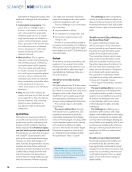
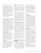
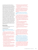
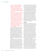
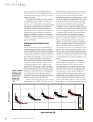
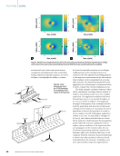
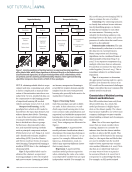
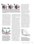
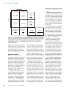
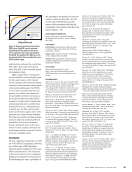
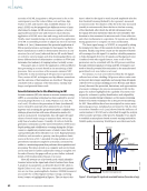
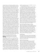
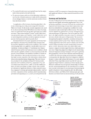
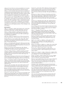
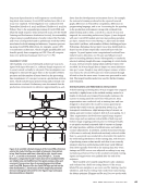
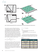
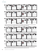
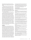
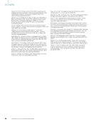
models, which are generally more inter- pretable (Figure 4). In essence, applying a model architecture should be inspired by the data and underlying factors at hand, especially for new datasets that have not been utilized for ML in the past. Metrics for Evaluation Evaluation metrics are performance measures for comparing ML models and understanding specific characteristics of the data or task. This is in part due to the bias and variance within the data. In particular, different evaluation metrics can be used to attain either a holistic performance or a class-specific measure. Here we review several of the most widely used metrics for evaluating the performance of ML models. Confusion matrix: The confusion matrix visualizes the predicted values against the true values. Elements on the diagonal of the matrix indicate the number of true predictions of the model to the true class (true positives and true negatives). The off-diagonal elements indicate incorrect predictions. Reading the confusion matrix tends to give further insight as to what types of errors are made for a model and allows a holistic set of evaluation metrics. We provide a typical illustration in Figure 5, together with the common name of such evaluation metrics. The confusion matrix need not be binary but can be con- ducted in a multi-class fashion. However, in the multi-class scenario, summarizing the model performance may be cum- bersome, and traditionally each class is evaluated in a one-versus-all manner. Accuracy: Accuracy is often the most common evaluation metric. The accuracy is the proportion of the model predictions correct relative to the true class. From the perspective of the confu- sion matrix, this is equivalent to the sum of the diagonal divided by the sum of all of the values. Accuracy is an easy value to understand. However, for imbalanced datasets, the accuracy can be uninforma- tive. For example, a common scenario in NDT/E might be that 99% of the data is from a normal material and 1% of the data is a material with a discontinuity. If 100% of the data is classified as normal, then the accuracy is 99%. This is often considered a good result until you recog- nize that none of the discontinuities are identified. Recall: Also known as sensitivity or the true positive rate (TPR), the recall is the proportion of true positive cases that are correctly predicted. In binary classifi- cation, notice that if 99% of the labels do not correspond to the class of interest, and 100% of the predictions correspond to those classes, then the recall will be 0. Hence, recall can be suitable when data is imbalanced. Precision: Also known as the positive predictive value (PPV), measures the proportion of correct positive predictions made. Observe, if 99% of the labels do not correspond to the class of interest, and 100% of the predictions correspond to those classes, then the precision will be 0. Therefore, precision can be advan- tageous when data is imbalanced. F1 score: The F1 score is a metric designed to summarize both preci- sion and recall. It is defined as the harmonic mean of precision and recall. The harmonic mean, as opposed to the arithmetic mean, addresses large devia- tions between precision and recall. For example, if the precision for a class is 0, and the recall is 1, then the arithme- tic mean evaluates to 0.5, which may naively indicate a random classifier. On the other hand, the harmonic mean in this scenario equates to 0, revealing the classifier is predicting only one class. Receiver operating characteristic curve: The receiver operating charac- teristic (ROC) curve can be generated when the confusion matrix varies as a function of a set call criterion (Figure 6). This metric originates from traditional statistical hypothesis testing in which a binary classifier is based upon the premise that some statistic is above or below a threshold. In a binary classifica- tion scenario, the ROC curve shows the false positive rate versus the true positive rate for all threshold values. To summa- rize the ROC, the area under the ROC curve (AUC) is often reported, where a perfect classifier attains a value of 1 and a random classifier attains an AUC of 0.5. The AUC metric is valuable as it is invariant of the chosen threshold Positive True positive (TP) Sensitivity true positive rate recall Specificity true negative rate Positive predictive Value |Precision Negative predictive value Accuracy F1-Score Negative True negative (TN) False negative (FN) Type II error False positive (FP) Type I error Predicted class TP TP +FN TP TP +FP TN TN +FP FP +FN TP +TN +FP +FN Precision × Recall Precision +Recall 2 × TN TN +FN Figure 5. A confusion matrix is used to evaluate the performance of a classifier, summarizing the information between true and predicted classifications. The confusion matrix entails the number of true positives, false negatives, false positives, and true negatives. Further classification metrics may be extracted (e.g., sensitivity, specificity, accuracy, etc.) to measure different aspects of the classifier. NDT TUTORIAL |AI/ML 46 M A T E R I A L S E V A L U A T I O N • J U L Y 2 0 2 3 2307 ME July dup.indd 46 6/19/23 3:41 PM Positive Negative T class

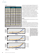
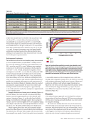
and therefore evaluates the overall clas- sifier rather than some user-chosen value. The AUC is also a feasible metric for imbalanced data. Tips: Careful choice of evaluation metrics should be selected based upon the bias and variance of the dataset. For an unbiased, well-balanced dataset, accuracy is often the most characteristic of the model performance. In NDT/E, we are often concerned with the true positive rate, which is also known as the probability of (defect) detection or the recall of a defect. In other NDT/E scenarios, we may want to ensure that normal materials are not predicted as material defects (e.g., delaminations), in which case, the false call rate (also known as the false negative rate) or the precision score may be more valuable. Note the true positive and false positive rates are utilized in traditional NDT/E probability of detection assessment (Cherry and Knott 2022). In the cases where we want a balance between the recall and precision scores, the F1 score becomes a valuable metric. Conclusion ML has a significant potential to contrib- ute to the NDT/E community. However, successful usage of ML algorithms demands greater insight into their capa- bilities and intricacies. This sentiment is also true for those in the community building new datasets for ML practices. Understanding the basic capabilities of ML paradigms, navigating how bias and variance within the data affect the ML model, and establishing how perfor- mance will be measured will help the community create datasets that have the greatest impact. ACKNOWLEDGMENTS Work on this paper is partially funded by the United States Air Force contract FA8650- 18-C-5015. AUTHORS Joel B. Harley: Department of Electrical and Computer Engineering, University of Florida, Gainesville, FL 32611 Suhaib Zafar: Stellantis Chrysler Technology Center, Auburn Hills, MI 48326 Charlie Tran: Department of Electrical and Computer Engineering, University of Florida, Gainesville, FL 32611 CITATION Materials Evaluation 81 (7): 43–47 https://doi.org/10.32548/2023.me-04358 ©2023 American Society for Nondestructive Testing REFERENCES Belkin, M., D. Hsu, S. Ma, and S. Mandal. 2019. “Reconciling modern machine-learning practice and the classical bias-variance trade-off.” Proceedings of the National Academy of Sciences of the United States of America 116 (32): 15849– 54. https://doi.org/10.1073/pnas.1903070116. Bishop, C. M. 2006. Pattern Recognition and Machine Learning. Springer New York. Brunton, S. L., B. R. Noack, and P. Koumout- sakos. 2020. “Machine Learning for Fluid Mechanics.” Annual Review of Fluid Mechanics 52 (1): 477–508. https://doi.org/10.1146/annurev- fluid-010719-060214. Cherry, M., and C. Knott. 2022. “What is proba- bility of detection?” Materials Evaluation 80 (12): 24–28. https://doi.org/10.32548/2022.me-04324. Du, M., N. Liu, and X. Hu. 2019. “Techniques for interpretable machine learning.” Commu- nications of the ACM 63 (1): 68–77. https://doi. org/10.1145/3359786. Lever, J., M. Krzywinski, and N. Altman. 2017. “Principal component analysis.” Nature Methods 14 (7): 641–42. https://doi.org/10.1038/ nmeth.4346. Liu, C., J. B. Harley, M. Bergés, D. W. Greve, and I. J. Oppenheim. 2015. “Robust ultrasonic damage detection under complex environ- mental conditions using singular value decom- position.” Ultrasonics 58:75–86. https://doi. org/10.1016/j.ultras.2014.12.005. Mann, L. L., T. E. Matikas, P. Karpur, and S. Krishnamurthy. 1992. “Supervised backpropa- gation neural networks for the classification of ultrasonic signals from fiber microcracking in metal matrix composites.” in IEEE 1992 Ultra- sonics Symposium Proceedings. Tucson, AZ. https://doi.org/10.1109/ULTSYM.1992.275983. Martín, Ó., M. López, and F. Martín. 2007. “Arti- ficial neural networks for quality control by ultrasonic testing in resistance spot welding.” Journal of Materials Processing Technology 183 (2–3): 226–33. https://doi.org/10.1016/j.jmat protec.2006.10.011. Mehrabi, N., F. Morstatter, N. Saxena, K. Lerman, and A. Galstyan. 2022. “A Survey on Bias and Fairness in Machine Learning.” ACM Computing Surveys 54 (6): 1–35. https://doi. org/10.1145/3457607. Miceli, M., J. Posada, and T. Yang. 2022. “Studying Up Machine Learning Data: Why Talk About Bias When We Mean Power?” Proc. ACM Hum.-Comput. Interact. 6: 1–14. https://doi. org/10.1145/3492853. OpenAI. 2023. “GPT-4 Technical Report.” arXiv:2303.08774. https://doi.org/10.48550/ arXiv.2303.08774. Saleem, M., and H. Gutierrez. 2021. “Using artificial neural network and non‐destructive test for crack detection in concrete surrounding the embedded steel reinforcement.” Structural Concrete 22 (5): 2849–67. https://doi.org/10.1002/ suco.202000767. Sikorska, J. Z., and D. Mba. 2008. “Challenges and obstacles in the application of acoustic emission to process machinery.” Proceedings of the Institution of Mechanical Engineers. Part E, Journal of Process Mechanical Engi- neering 222 (1): 1–19. https://doi.org/10.1243/ 09544089JPME111. Taheri, H., and S. Zafar. 2023. “Machine learning techniques for acoustic data processing in additive manufacturing in situ process monitoring — A review.” Materials Evaluation 81 (7): 50–60. Taheri, H., M. Gonzalez Bocanegra, and M. Taheri. 2022. “Artificial Intelligence, Machine Learning and Smart Technologies for Nonde- structive Evaluation.” Sensors (Basel) 22 (11): 4055. https://doi.org/10.3390/s22114055. van der Maaten, L., and G. Hinton. 2008. “Visu- alizing Data using t-SNE.” Journal of Machine Learning Research 9 (86): 2579–605. Vejdannik, M., A. Sadr, V. H. C. de Albu- querque, and J. M. R. S. Tavares. 2019. “Signal Processing for NDE,” in Handbook of Advanced Nondestructive Evaluation. eds. N. Ida and N. Meyendorf. Springer. pp. 1525–1543. https://doi. org/10.1007/978-3-319-26553-7_53. Xu, D., P. F. Liu, Z. P. Chen, J. X. Leng, and L. Jiao. 2020. “Achieving robust damage mode identification of adhesive composite joints for wind turbine blade using acoustic emission and machine learning.” Composite Structures 236:111840. https://doi.org/10.1016/j.comp- struct.2019.111840. Yang, K., S. Kim, and J. B. Harley. 2022. “Guide- lines for effective unsupervised guided wave compression and denoising in long-term guided wave structural health monitoring.” Structural Health Monitoring. https://doi. org/10.1177/14759217221124689. 1.0 0.5 0.0 0.5 1.0 False positive rate Excellent classifier Good classifier Random classifier AUC Figure 6. Receiver operating characteristic (ROC) curve. The ROC curve is achieved by plotting the false positive rate versus the true positive rate at each classification threshold. The quality of the ROC curve can be summarized by the area under the curve (AUC) shaded in gray. J U L Y 2 0 2 3 • M A T E R I A L S E V A L U A T I O N 47 2307 ME July dup.indd 47 6/19/23 3:41 PM T positive rate