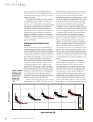
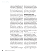
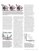
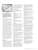
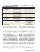
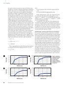
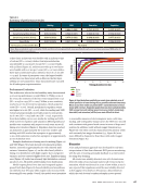
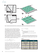
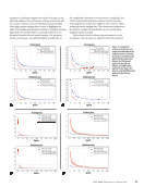
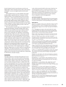
a batch size of 32, with early stopping and learning rate reduc- tion based on validation loss. Binary cross-entropy loss was used for the event outputs, while mean-squared error was used on the MNS regression output. Inputs and loss were masked such that models would skip the zero-vector A-scans during training and not backpropagate loss on those inputs thus, the model did not learn from the zero-padded regions. To evaluate performance, a number of different perfor- mance indicators were used for each task. With respect to event detection, performance was evaluated using sensitivity with respect to the absolute error of ground truth versus model predictions of event timings from 0–30 ms, overall specific- ity, and histograms of timing error for true positives. MNS regression performance was assessed using the percentage of A-scans that are correct within an absolute difference of 0.1. Results The results of the feasibility study and performance evaluation are discussed next. Feasibility Study The feasibility study results (Table 1) demonstrated that archi- tectures starting with eight filters in the first layer were feasible up to three layers (Figure 5a). The three-layer architecture with eight filters in the first layer had an inference time of 1.06 ms (SD =0.13 ms), whereas a four-layer architecture had an infer- ence time of 1.22 ms (SD =0.14 ms). With 16 filters (Figure 5b), ME |AI/ML T A B L E 1 Summary of feasibility study results Architecture (filters per ConvLSTM layer) Parameters Inference time (ms) 8 3461 0.866 (0.193) 8-16 8133 1.024 (0.155) 8-16-32 26 693 1.060 (0.129) 8-16-32-64 100 677 1.221 (0.142) 8-16-32-64-128 396 101 1.428 (0.155) 16 8453 0.952 (0.304) 16-32 27 013 0.954 (0.160) 16-32-64 100 997 1.085 (0.151) 16-32-64-128 396 421 1.344 (0.132) 16-32-64-128-256 1 577 093 1.992 (0.154) 32 23 045 0.999 (0.268) 32-64 97 029 0.970 (0.108) 32-64-128 392 453 1.264 (0.126) 32-64-128-256 1 573 125 1.942 (0.144) 32-64-128-256-512 6 293 765 4.271 (0.189) Note: Mean inference time per A-scan over 2589 A-scans, standard deviation in parentheses Architecture Architecture Architecture Legend Inference time Parameters 8 8-16 8-16-32 8-16-32-64 8-16-32-64-128 400 000 300 000 200 000 100 000 0 4.5 4 3.5 3 2.5 2 1.5 1 0.5 0 6 000 000 4 000 000 2 000 000 0 32 32-64 32-64-128 32-64-128-256 32-64-128-256-512 4.5 4 3.5 3 2.5 2 1.5 1 0.5 0 16 16-32 16-32-64 16-32-64-128 16-32-64-128-256 1 600 000 1 200 000 800 000 400 000 0 4.5 4 3.5 3 2.5 2 1.5 1 0.5 0 Figure 5. Inference time per A-scan in milliseconds (orange line) and parameter count (blue dashed line) per architecture (X axis 1–5 layers), with first layer number of filters: (a) 8 (b) 16 and (c) 32. Inference time generally grows superlinearly with respect to both number of layers and parameters. Means across all 2589 A-scans are plotted with 1 standard deviation of mean shown with error bars. 66 M A T E R I A L S E V A L U A T I O N • J U L Y 2 0 2 3 2307 ME July dup.indd 66 6/19/23 3:41 PM No .of parameter s N o. of parameters No .of parameter s A-scan inference time (ms) A-scan inference time (ms) A-scan inference time (ms)

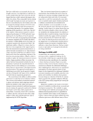
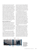
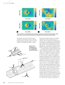
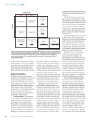
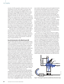
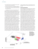
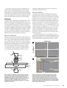
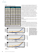
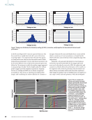
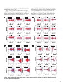
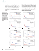
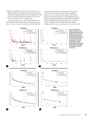
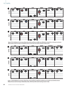
a three-layer architecture was feasible with an inference time of 1.08 ms (SD =0.15 ms), while a four-layer architecture was infeasible at 1.34 ms per A-scan (SD =0.13 ms). Finally, with 32 filters (Figure 5c), architectures with up to two layers were feasible with 0.97 ms per A-scan (SD =0.27 ms), while a three-layer architecture had an inference time of 1.26 ms (SD =0.13 ms). In terms of parameter count, the largest feasible architecture was three layers with 16 filters in the first layer, yielding 100 997 parameters. Thus, this architecture was used for all subsequent experimentation. Performance Evaluation The architecture selected in the feasibility study demonstrated a very strong performance overall (Table 2). Within 10 ms of the event, the sensitivity of the four events ranged from 0.742 (SD =0.023) to 0.935 (SD =0.005). Within 30 ms, sensitivity reached 0.977 for all events but saturation, which peaked at 0.898 (SD =0.009). Overall, specificity for expulsion events was highest at 0.986 (SD =0.002), while the melting and SSID events had proportionally more false positives with specific- ity of 0.807 (SD =0.025) and 0.821 (SD =0.031), respectively. Event detectability curves were similar for melting and SSID, while curves for expulsion and saturation differed greatly and models were consistent with respect to each event across all timing error windows (Figure 6). Expulsion detection reached an asymptote at approximately the 5 ms error window and melting and SSID reached an asymptote at approximately 15 ms, while saturation reached an asymptote at approximately 30 ms of absolute error. Example distributions of timing error for melting (Figure 7a) and SSID (Figure 7b) events showed very symmetrical distri- butions, centered at approximately zero with relatively mild variance. Saturation (Figure 7c), on the other hand, yielded a timing error distribution with slight negative skew and greater variance, and was centered slightly above zero. Expulsion timing error (Figure 7d) yielded an extremely tight distribution centered just above zero. All models yielded similar error distributions. Model outputs plotted over time and compared against ground truth data (Figure 8) showed stability and smoothness on relatively clear M-scans, while output noise increased with decreasing M-scan quality. Overall, the models were insensitive to reasonable amounts of electromagnetic noise, weld time, stackup, and weld quality. Output curves for MNS were smooth and consistent with ground truth curves in terms of shape and position. In addition, welds without nugget formation (e.g., Figure 8a) were often correctly characterized. In general, welds with extremely late nugget formation (e.g., Figure 8b) were more difficult to characterize than those with earlier nugget formation (Figure 8c). Discussion A fast and performant approach was developed for real-time interpretation of data from ultrasonic RSW process monitoring, with the aim of creating actionable feedback to a weld control- ler using deep learning. All events were reliably detected over 95% of events were detected within 18 ms of ground truth for all events except for saturation, which was detected at a rate of 90% within 30 ms. It was expected that expulsions would be most reliably detected as they appear very clearly on M-scans as a discontinuity in which the stack bottom boundary abruptly moves upward T A B L E 2 Summary of performance results Melting SSID Saturation Expulsion Sensitivity (within 10 ms) 0.870 (0.010) 0.886 (0.009) 0.742 (0.023) 0.935 (0.005) Sensitivity (within 20 ms) 0.963 (0.006) 0.962 (0.007) 0.860 (0.014) 0.954 (0.006) Sensitivity (within 30 ms) 0.984 (0.003) 0.979 (0.002) 0.898 (0.009) 0.977 (0.001) Specificity 0.807 (0.025) 0.821 (0.031) 0.933 (0.018) 0.986 (0.002) %A-scans correct (within 0.1) 90.5 (0.4) Note: Mean sensitivity for each event within 10, 20, and 30 ms of event ground truth, mean specificity for each event, and mean accuracy of MNS within 0.1. Standard deviation in parentheses. Figure 6. Event detection sensitivity per event given absolute error of model prediction of event timing versus ground truth event timestamp. Means across three models are plotted with 1 standard deviation of mean shown with error bars. Expulsion (purple line) was most easily detectable, SSID (orange line) and melting (green line) were similarly moderately detectable, and saturation (red line) was most difficult to detect. Timing absolute error (ms) Legend Melting SSID Saturation Expulsion 1 0.9 0.8 0.7 0.6 0.5 0.4 0.3 0.2 0.1 0 0 5 10 15 20 25 30 J U L Y 2 0 2 3 • M A T E R I A L S E V A L U A T I O N 67 2307 ME July dup.indd 67 6/19/23 3:41 PM Sensitivity