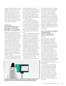
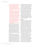
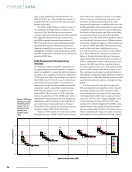
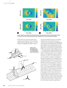
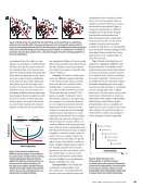
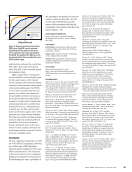
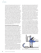
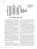
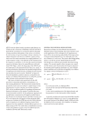
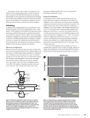
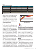
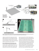
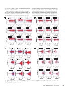
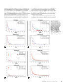
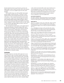
edges of the plate, respectively. Utilizing FEM simulations, we generated waveforms from nine distinct locations similar to the experimental setup shown in Figure 2. Simulating AE signals via FEM allows us to generate pretraining data for deep learning models, thereby enabling a more accurate and efficient localization of acoustic emission sources within the specimen. These simulated signals furnish an effective means to pretrain deep learning models for AE signal processing algo- rithms, consequently bolstering the accuracy and effectiveness of these algorithms in real-world contexts. For the PLB test, the excitation signal, ​​ ​ 1​​​(t)​​ simulates the response of an aluminum plate to mechanical loading and is defined as follows: ​ ​ F1​​​(t)​ ​ =​ {​ − 2t/​t​1​​, 0 x ​ t1​​​ ​ − cos​ π[t ​ − ​ t​1​​]​)​ − 1, ​ t​1​​ x ​ t​2​​​ 0,​t​2​​ x ​ ​ ​ The function was selected due to its ability to elicit a gradual increase in the excitation signal. Here, ​​ ​ 1​​​ and ​​ ​ 2​​​ are time inter- vals that define specific stages of the excitation signal. ​​ ​ 1​​​ sig- nifies the duration over which the excitation signal increases gradually, while ​​ ​ 2​​​ denotes the time after which the signal ceases. This particular function was chosen as it prompts a gradual increase in the excitation signal, thus adequately repre- senting the mechanical loading process. For the impact test, ​​ ​ 2​​​ (t)​​ is represented as: ​ ​ F​2​​​(t)​ =C ​ e​​ −γt/​t​0​​​ sin​ (​ 4π _1 +​​ t​0​​ t ​ ​ ​​ where C is the initial amplitude of the excitation signal, γ is the damping factor, ​ ​ t​0​​​ is the characteristic time of the excitation signal, and t is time. This function, representing a damped sinusoidal wave, is a common signal observed in impact tests and serves to simulate the material response to mechanical loading. The shape of the ​ ​ 0 –0.2 –0.4 –0.6 –0.8 –1 –1.2 –1.4 –1.6 –1.8 –2 0.8 0.6 0.4 0.2 0 –0.2 –0.4 0 2 4 6 8 10 Time (μs) 0 2 4 6 8 10 Time (μs) z y x z y x Sensor 12 in. 12 in. Sensor Zone 1 Zone 4 Zone 5 Zone 6 Zone 9 Zone 8 Zone 7 Zone 2 Zone 3 Zone 1 Zone 4 Zone 5 Zone 6 Zone 9 Zone 8 Zone 7 Zone 2 Zone 3 Ramp function Impact source Figure 3. Simulation setup with analytical functions: (a) excitation signal to simulate PLB test (b) excitation signal to simulate impact test. T A B L E 1 Parameters for simulation Parameters Values Young’s modulus 206 GPa Poisson’s ratio 0.3 Density 2710 kg/m3 t0 5 μs t1 6.5 μs t2 7.5 μs Decay rate γ 1.85 ME |AI/ML 74 M A T E R I A L S E V A L U A T I O N • J U L Y 2 0 2 3 2307 ME July dup.indd 74 6/19/23 3:41 PM Amplitude (N) Amplitude (N)

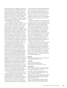
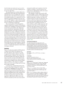
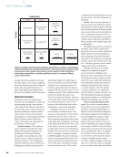
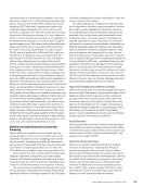
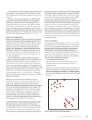
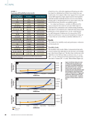
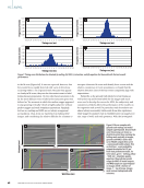
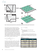
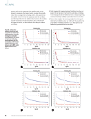
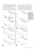
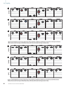
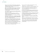
F​1​​​(t)​​ and ​ ​ F​2​​​(t)​ ​ shown in Figure 3 and specifications of these parameters are shown in Table 1. Figure 4 showcases the signals derived from the impact and PLB tests and their corresponding simulation signals. We present these waveforms to emphasize the clear correlations and dissimilarities between test and simulation data such contrasts highlight the feasibility of employing deep learning models in acoustic emission source localization. The duration of these signals is distinct for the tests and simulations the test signals span a duration of 250 μs, while the simulation signals extend over a period of 100 μs. This discrepancy is a consequence of the methods employed to gather sufficient Location 2 Location 3 Location 4 Location 5 Location 6 Location 7 Location 8 Location 9 4 2 0 –2 –4 0 100 200 Time (μs) 4 2 0 –2 –4 0 100 200 Time (μs) 2 0 –2 –4 0 100 200 Time (μs) 2 0 –2 –4 0 100 200 Time (μs) 4 2 0 –2 –4 0 100 200 Time (μs) 4 2 0 –2 –4 0 100 200 Time (μs) 4 2 0 –2 –4 0 100 200 Time (μs) 4 2 0 –2 –4 0 50 100 Time (μs) 4 2 0 –2 –4 0 50 100 Time (μs) 4 2 0 –2 –4 0 50 100 Time (μs) 4 2 0 –2 –4 0 50 100 Time (μs) 4 2 0 –2 –4 0 50 100 Time (μs) 4 2 0 –2 –4 0 100 200 Time (μs) 4 2 0 –2 –4 0 100 200 Time (μs) 5 0 –5 0 50 100 Time (μs) 5 0 –5 0 100 200 Time (μs) 5 0 –5 0 100 200 Time (μs) 5 0 –5 0 100 200 Time (μs) 5 0 –5 0 100 200 Time (μs) 5 0 –5 0 100 200 Time (μs) 5 0 –5 0 100 200 Time (μs) 5 0 –5 0 100 200 Time (μs) 5 0 –5 0 100 200 Time (μs) 5 0 –5 0 100 200 Time (μs) 5 0 –5 0 50 100 Time (μs) 5 0 –5 0 50 100 Time (μs) 5 0 –5 0 50 100 Time (μs) 5 0 –5 0 50 100 Time (μs) 5 0 –5 0 50 100 Time (μs) 5 0 –5 0 50 100 Time (μs) 5 0 –5 0 50 100 Time (μs) 5 0 –5 0 50 100 Time (μs) 5 0 –5 0 50 100 Time (μs) 6 4 2 0 –2 –4 0 50 100 Time (μs) 6 4 2 0 –2 –4 0 50 100 Time (μs) 6 4 2 0 –2 –4 0 50 100 Time (μs) Location 1 Location 2 Location 3 Location 4 Location 5 Location 6 Location 7 Location 8 Location 9 Location 1 Location 2 Location 3 Location 4 Location 5 Location 6 Location 7 Location 8 Location 9 Location 1 Location 2 Location 3 Location 4 Location 5 Location 6 Location 7 Location 8 Location 9 Location 1 Figure 4. Signals obtained from: (a) impact test (b) PLB test (c) impact simulation and (d) PLB simulation. The raw signal is denoted in blue, while the red line signifies the average waveform. J U L Y 2 0 2 3 • M A T E R I A L S E V A L U A T I O N 75 2307 ME July dup.indd 75 6/19/23 3:41 PM Voltage (V) Voltage (V) Voltage (V) Voltage (V) Voltage(V) Voltage(V) Voltage(V) Voltage (V) Voltage (V) Voltage (V) Voltage (V) Voltage (V) Voltage(V) Voltage(V) Voltage (V) Voltage(V) Voltage (V) Voltage (V) Voltage (V) Voltage (V) Voltage (V) Voltage (V) Voltage(V) Voltage(V) Voltage (V) Voltage (V) Voltage (V) Voltage (V) Voltage(V) Voltage(V) Voltage(V) Voltage (V) Voltage (V) Voltage (V) Voltage (V) Voltage (V)