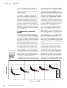
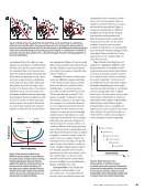
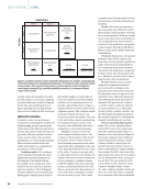
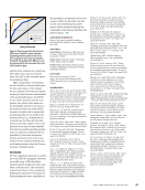
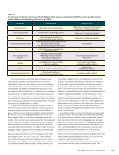
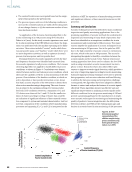
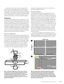
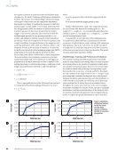
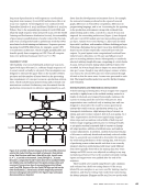
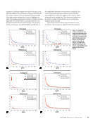
on simulated data (for which we can produce an abundance of labeled data) will learn the specific characteristics of the simulated data, but it may not also represent experimentally measured data. If the labels are imbalanced (e.g., there are twice as many cracks as delamina- tions), then the data will be inherently more likely to predict the larger class. In short, if a characteristic of our data is imbalanced (e.g., twice as many mea- surements originate from aircraft wings than bridges), then the predictions will be more accurate for those dominant characteristics. An underfit ML model is created when trained with a biased dataset or when the ML model has too few parameters (Figure 2). Such a model fails to learn specific characteristics from the data, leading to poor performance (the classic bias-variance tradeoff is illus- trated in Figure 3). Variance: The effects of data imbal- ances are difficult to gauge in part due to the variance in the dataset, another factor that must be considered when building data. A common question posed by non-ML practitioners is often “How much data do you need?” The answer is usually “it depends” due to the inherent variance in the input data. For example, if a crack looks identical in every single measurement, then the dataset has very low variance. In this scenario, you may not need a learning system because one datum of a crack sufficiently describes all other examples (although some pattern recognition is still necessary). In contrast, if there are a million different and unique permuta- tions of how a crack is represented, then the ML model will need at least a million examples to correctly classify cracks. In reality, there are usually complex rela- tionships between all data correspond- ing to cracks, which the ML model can learn. A highly variable dataset with too few training examples and too many parameters to learn can yield an overfit ML model (Figure 2). Such a model may find uninformative relationships in noise, leading to poor performance (Figure 3) (Belkin et al. 2019). Interpretability: One should also consider the interpretability of an ML architecture. An interpretable ML model is one from which humans can comprehend how a decision is made (Du et al. 2019). In general, there is a negative correlation between accuracy and model interpretability (Figure 4). Gaining interpretability is a difficult problem due to the nature of black- box models, non-linearities, and high-dimensional data visualizations. Deep neural networks are the prime example, being the most accurate models but with little to no interpretabil- ity of the model decision-making. On the other hand, linear models (e.g., linear regression) are very interpretable, yet often less accurate. Tips: Misunderstanding bias and variance is a significant pitfall for early ML practitioners. For example, novice deep learning practitioners often default toward increasing the number of layers in a neural network, thereby increasing the model complexity. However, such an architecture is not only more compu- tationally demanding but can in some cases be less effective (due to overfitting) and less interpretable than a simpler architecture. For this reason, deep neural networks are unfavorable in situations with limited data samples of potentially high variance and situations where interpretability and accountability are important. In such a scenario, users may often analyze their problem using con- ventional ML models, such as support vector machines or linear regression Figure 2. Model fitting: (a) underfitting (b) ideal fitting and (c) overfitting. An underfitting model characteristically suffers from poor performance in the training data, being unable to learn the relationships within the data. On the other hand, an overfitting model characteristically suffers from over-performing on the training data (often viewed as “memorization”) and fails to generalize onto new data samples. Thus, a fundamental goal of machine learning algorithms is to find an ideal fitting. High bias Low variance Underfitting Low bias High variance Overfitting Optimal Variance Generalization error Bias2 Model complexity Figure 3. Bias-variance tradeoff curve. Machine learning models strive to balance bias and variance. Simple machine learning models typically have fewer parameters, wherein the high bias and low variance are characteristic of model underfitting. On the other hand, complex machine learning models have a large number of parameters, wherein the low bias and high variance are characteristic of model overfitting. Deep neural networks High High Low Random forests Support vector machines K-nearest-neighbors Decision trees Linear regression Interpretability Figure 4. Model accuracy versus interpretability. In machine learning, increased accuracy has a natural consequence of decreased interpretability. Accurate models tend to capture nonlinear and non-smooth relationships, while interpretable models tend to capture linear and smooth relationships. J U L Y 2 0 2 3 • M A T E R I A L S E V A L U A T I O N 45 2307 ME July dup.indd 45 6/19/23 3:41 PM Prediction error Accuracy

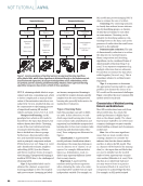
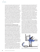
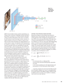
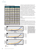
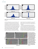
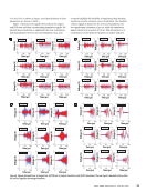
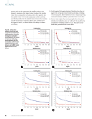
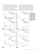
models, which are generally more inter- pretable (Figure 4). In essence, applying a model architecture should be inspired by the data and underlying factors at hand, especially for new datasets that have not been utilized for ML in the past. Metrics for Evaluation Evaluation metrics are performance measures for comparing ML models and understanding specific characteristics of the data or task. This is in part due to the bias and variance within the data. In particular, different evaluation metrics can be used to attain either a holistic performance or a class-specific measure. Here we review several of the most widely used metrics for evaluating the performance of ML models. Confusion matrix: The confusion matrix visualizes the predicted values against the true values. Elements on the diagonal of the matrix indicate the number of true predictions of the model to the true class (true positives and true negatives). The off-diagonal elements indicate incorrect predictions. Reading the confusion matrix tends to give further insight as to what types of errors are made for a model and allows a holistic set of evaluation metrics. We provide a typical illustration in Figure 5, together with the common name of such evaluation metrics. The confusion matrix need not be binary but can be con- ducted in a multi-class fashion. However, in the multi-class scenario, summarizing the model performance may be cum- bersome, and traditionally each class is evaluated in a one-versus-all manner. Accuracy: Accuracy is often the most common evaluation metric. The accuracy is the proportion of the model predictions correct relative to the true class. From the perspective of the confu- sion matrix, this is equivalent to the sum of the diagonal divided by the sum of all of the values. Accuracy is an easy value to understand. However, for imbalanced datasets, the accuracy can be uninforma- tive. For example, a common scenario in NDT/E might be that 99% of the data is from a normal material and 1% of the data is a material with a discontinuity. If 100% of the data is classified as normal, then the accuracy is 99%. This is often considered a good result until you recog- nize that none of the discontinuities are identified. Recall: Also known as sensitivity or the true positive rate (TPR), the recall is the proportion of true positive cases that are correctly predicted. In binary classifi- cation, notice that if 99% of the labels do not correspond to the class of interest, and 100% of the predictions correspond to those classes, then the recall will be 0. Hence, recall can be suitable when data is imbalanced. Precision: Also known as the positive predictive value (PPV), measures the proportion of correct positive predictions made. Observe, if 99% of the labels do not correspond to the class of interest, and 100% of the predictions correspond to those classes, then the precision will be 0. Therefore, precision can be advan- tageous when data is imbalanced. F1 score: The F1 score is a metric designed to summarize both preci- sion and recall. It is defined as the harmonic mean of precision and recall. The harmonic mean, as opposed to the arithmetic mean, addresses large devia- tions between precision and recall. For example, if the precision for a class is 0, and the recall is 1, then the arithme- tic mean evaluates to 0.5, which may naively indicate a random classifier. On the other hand, the harmonic mean in this scenario equates to 0, revealing the classifier is predicting only one class. Receiver operating characteristic curve: The receiver operating charac- teristic (ROC) curve can be generated when the confusion matrix varies as a function of a set call criterion (Figure 6). This metric originates from traditional statistical hypothesis testing in which a binary classifier is based upon the premise that some statistic is above or below a threshold. In a binary classifica- tion scenario, the ROC curve shows the false positive rate versus the true positive rate for all threshold values. To summa- rize the ROC, the area under the ROC curve (AUC) is often reported, where a perfect classifier attains a value of 1 and a random classifier attains an AUC of 0.5. The AUC metric is valuable as it is invariant of the chosen threshold Positive True positive (TP) Sensitivity true positive rate recall Specificity true negative rate Positive predictive Value |Precision Negative predictive value Accuracy F1-Score Negative True negative (TN) False negative (FN) Type II error False positive (FP) Type I error Predicted class TP TP +FN TP TP +FP TN TN +FP FP +FN TP +TN +FP +FN Precision × Recall Precision +Recall 2 × TN TN +FN Figure 5. A confusion matrix is used to evaluate the performance of a classifier, summarizing the information between true and predicted classifications. The confusion matrix entails the number of true positives, false negatives, false positives, and true negatives. Further classification metrics may be extracted (e.g., sensitivity, specificity, accuracy, etc.) to measure different aspects of the classifier. NDT TUTORIAL |AI/ML 46 M A T E R I A L S E V A L U A T I O N • J U L Y 2 0 2 3 2307 ME July dup.indd 46 6/19/23 3:41 PM Positive Negative T class