axial and radial magnetic leakage field, and to obtain the rela-
tionship between the edge angle of discontinuities of differ-
ent shapes and the changes in magnetic leakage signals. To
simplify the calculation, a steel plate is used as the test sample,
with artificial defects machined on its surface to simulate real
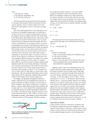
conditions, as shown in Figure 2. The model includes a mild
steel sample, an excitation coil, a soft iron yoke, a Hall element,
and an artificial defect. The material properties of each part are
listed in Table 1.
In particular, when grid dissection is performed using
COMSOL software, focused calculations and grid encryption
are applied near the surface on the defect side to improve
the smoothness and accuracy of the leakage field acquisition
results.
Magnetic Leakage Signal Analysis of Discontinuities
with Different Edge Angles
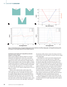
In engineering, the edge angles of discontinuities can vary
arbitrarily between 0° and 180°. This paper focuses on the
study of discontinuity edge angles in the range of 0° to 90°, as
these angles are more common in actual working conditions.
Based on the principle of magnetic leakage detection and
COMSOL simulation, this paper presents several discontinuity
models and further investigates the characteristic relationship
between the edge angles of these discontinuity models and the
magnetic leakage signal.
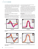
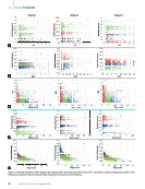
Selection of Liftoff Values in Leakage Detection
The choice of liftoff value is one of the key factors affecting
the acquisition of a magnetic leakage signal. A suitable liftoff
value should be selected based on the actual detection of the
component. If the liftoff value is too small, friction may occur
with the sensor during the moving detection process, thus
shortening the service life of the sensor. Similarly, if the liftoff
value is too large, the signal collected by the sensor will be
weak and the sensor may not be sensitive to magnetic leakage
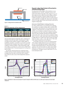
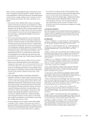
signals. Therefore, a right-angled trapezoidal discontinuity with
an edge angle of 63° is taken as the object of study, with liftoff
values of 0.2 mm, 0.5 mm, 0.7 mm, and 1 mm set. The results
of the simulated signals are shown in Figure 3.
From Figures 3a and 3b, it can be seen that the intensity
of the magnetic leakage signal decreases as the liftoff value
increases. The radial and axial magnetic leakage signals are
strongest when the liftoff value is 0.2 mm. Practical consid-
erations for the experimental process suggest using a higher
liftoff value to better protect the sensors from damage (Sun
and Kang 2010). This paper chooses a liftoff value of 0.5 mm
for the subsequent study.
Artificial
defect
Hall element
Soft iron yoke
Excitation coil
Low-carbon steel
Figure 2. Leakage detection simulation model.
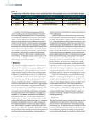
TA B L E 1
Material properties of the components
Part Material Relative
permeability
Conductivity
(S/m)
Sample Carbon steel 400 8.41 ​ ​ 107
Excitation coil Copper 1 5.99 ​ 107
Yoke Soft iron 4000 1.12 ​ 107
80
70
60
50
40
40
50
60
70
80
90
100
110
120
30
30
20
10
–10
–20
–30
–40
–50
–60
–70
–80
–90
–100
0
0 5 10
Scanning path (mm) Scanning path (mm)
15 20 0 5 10 15 20
0.2 mm
0.5 mm
0.7 mm
1 mm
0.2 mm
0.5 mm
0.7 mm
1 mm
Figure 3. Distribution of radial and axial signals of magnetic leakage for different liftoff values: (a) radial signal component (b) axial signal
component.
M AY 2 0 2 5 • M AT E R I A L S E V A L U AT I O N 33
B
(mT)
B
(mT)

Simulation and Analysis of V-shaped Discontinuity
Magnetic Leakage Signal
Under normal conditions, when the sample to be tested is
magnetized, the magnetic lines of force are evenly distrib-
uted inside the sample. When a discontinuity is present, the
magnetic lines of force leak and generate a leakage magnetic
field at the discontinuity’s edge. As shown in Figure 4a, using a
V-shaped discontinuity as an example, the width of the discon-
tinuity is determined to be 4 mm, the thickness of the sample
is 5 mm, and the edge angles are 20°, 45°, and 65°, in that
order. The variation in the magnetic leakage signal is shown in
Figures 4c and 4d.
Figure 4c shows that the peak-to-peak values of the
radial component of the discontinuities gradually increase
as the edge angle increases. Meanwhile, the peak point of
the magnetic leakage signal becomes progressively wider in
the horizontal direction relative to the center position of the
discontinuity as the edge angle changes from 20° to 65°. The
peak value of the waveform of the axial signal in Figure 4d also
increases with the increase of the edge angle. Assuming the
discontinuity width remains constant, the change in the hori-
zontal direction of the axial signal is consistent with the change
in the radial signal.
From Figure 4b, it can be seen that the signal peak grad-
ually increases as the edge angle increases. Additionally,
relative to the center position of the discontinuity at 10 mm,
the larger the edge angle, the farther the peak point moves
from the center. This indicates that as α increases, the value of
sin(​​ ​ 1​​ − α​ decreases. As a result, the refraction angle ​​ ​ 2​​​ of the
magnetic field lines decreases, causing the refracted magnetic
field lines at the media interface to approach the normal of
the interface. This leads to a denser concentration of refracted
magnetic field lines. Consequently, the magnetic field lines
after refraction become more concentrated, resulting in a
larger magnetic induction intensity (B) for both the axial and
radial signals. The peak-to-peak spacing also increases.
This study also observed changes in the depth of the dis-
continuities, highlighting the need for further research on the
correlation between the variable edge angle and the magnetic
leakage signal.
ME
|
MAGNETICLEAKAGE
80
100
60
40
40
50
60
70
80
90
100
110
120
130
140
150
160
0
20
40
60
80
9.2
9.0
8.8
8.6
8.4
8.2
8.0
7.8
100
20
–20
–40
–60
–80
–100
0
0 5 10
Scanning path (mm) Scanning path (mm)
15 20 0 5 10
Edge angle (degrees)
45°
45°
20°
20°
65°
65°
15 20
65°
45°
20°
65°
45°
20°
Figure 4. V-shaped discontinuity and magnetic leakage signal variation distribution for different edge angles: (a) V-shaped discontinuity model
(b) trend plot (c) radial signal component (d) axial signal component.
34
M AT E R I A L S E V A L U AT I O N • M AY 2 0 2 5
B
(mT)
B
(mT)
B
(mT)
L
point