Simulation and Analysis of Trapezoidal Discontinuity
Magnetic Leakage Signal
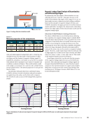
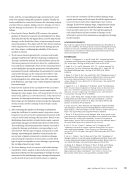
It was shown that there is indeed a link between the disconti-
nuity edge angle and the magnetic leakage signal, which is par-
ticularly evident in the radial component. To further determine
the effect of edge angle on the magnetic leakage signal, the
study continued with other discontinuity models. These were
changed to rectangular and right-angle trapezoidal disconti-
nuities, with a width of 4 mm, a depth of 2 mm, and a sample
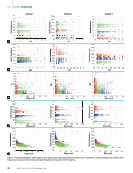
thickness of 5 mm. As shown in Figure 5a, a constant angle of
90° was maintained on one side of the discontinuity, while the
edge angles on the other side were 39°, 45°, 53°, 63°, 76°, and
90°, respectively.
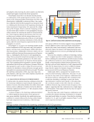
As shown in Figures 5b and 5c, the radial magnetic leakage
signal changes as the edge angle changes. The specific trend
is that as the edge angle increases, the peak intensity of the
radial signal increases, and the distance from the peak point
to the center of the discontinuity becomes wider. The increase
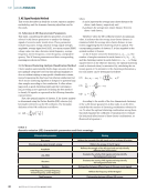
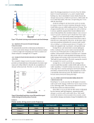
in peak value accelerates as the edge angle increases. A regres-
sion analysis was performed on the edge angle and peak point,
and the results are shown in Table 2.
As can be seen from the table, the multiple R-value is
about 0.976, which exceeds 0.75, indicating a strong correla-
tion between the size of the edge angle and the location of the
signal peak (Domenech-Asensi et al. 2005). The regression
equation can be expressed as follows:
(10) y =8.3889 − 0.0063x
where
the independent variable is the edge angle magnitude, and
y is the location of the peak point of the radial magnetic
leakage signal.
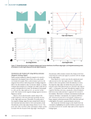
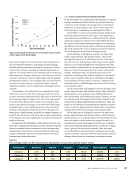
Figure 5d illustrates that variations in the edge angles
influence the amplitude of the axial signal. Specifically, the
larger the edge angle, the larger the amplitude. As the edge
angle increases, the axial signal gradually transitions from a
single wave peak to a double wave peak. The reasons for this
are explained as follows.
The refraction angle 2 of the magnetic field lines at the dis-
continuity boundary decreases due to the increased influence
of the edge angle α on the magnetic field lines. This causes the
propagation of the magnetic field lines to become more centrally
TA B L E 2
Relationship between edge angle and peak position
Regression statistics
Multiple R 0.976070929
R-square 0.952714458
Adjusted R-square 0.940893073
Standard error 0.030167813
Observed value 6
39° 45° 53°
63° 76° 90°
60 8.20
8.15
8.10
8.05
8.00
7.95
7.90
7.85
40
30
20
50
10
–20
–30
–10
–40
–50
–60
0
0 39° 45° 53° 63° 76° 90° 5 10
Scanning path (mm) Edge angle (degrees)
15 20
60
70
80
90
100
110
120
130
140
150
40
30
20
50
0 5 10
Scanning path (mm)
15 20
40
50
60
70
80
90
100
110
120
0 5 10
Scanning path (mm)
40
45
30
35
50
55
60
65
15 20
35
40
45
50
55
60
65
70
75
80
85
90
95
100
0 5 10
Scanning path (mm)
15 20
90°
76°
63°
53°
45°
39°
90°
76°
63°
53°
45°
39°
3 A
4 A
5 A
6 A
7 A
1 mm
2 mm
3 mm
4 mm
5 mm
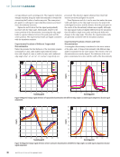
Figure 5. Trapezoidal discontinuity and magnetic leakage signal distributions under different conditions: (a) trapezoidal discontinuity model
(b) trend plot (c) radial signal components at different edge angles (d) axial signal components at different edge angles (e) axial signal
components at the same edge angle for different discontinuity widths (f) axial signal components at the same edge angle for different
magnetizing currents.
M AY 2 0 2 5 • M AT E R I A L S E V A L U AT I O N 35
B
(mT)
B
(mT)
B
(mT)
B
(mT)
B
(mT)
L
point
Magnetic Leakage Signal
It was shown that there is indeed a link between the disconti-
nuity edge angle and the magnetic leakage signal, which is par-
ticularly evident in the radial component. To further determine
the effect of edge angle on the magnetic leakage signal, the
study continued with other discontinuity models. These were
changed to rectangular and right-angle trapezoidal disconti-
nuities, with a width of 4 mm, a depth of 2 mm, and a sample
thickness of 5 mm. As shown in Figure 5a, a constant angle of
90° was maintained on one side of the discontinuity, while the
edge angles on the other side were 39°, 45°, 53°, 63°, 76°, and
90°, respectively.
As shown in Figures 5b and 5c, the radial magnetic leakage
signal changes as the edge angle changes. The specific trend
is that as the edge angle increases, the peak intensity of the
radial signal increases, and the distance from the peak point
to the center of the discontinuity becomes wider. The increase
in peak value accelerates as the edge angle increases. A regres-
sion analysis was performed on the edge angle and peak point,
and the results are shown in Table 2.
As can be seen from the table, the multiple R-value is
about 0.976, which exceeds 0.75, indicating a strong correla-
tion between the size of the edge angle and the location of the
signal peak (Domenech-Asensi et al. 2005). The regression
equation can be expressed as follows:
(10) y =8.3889 − 0.0063x
where
the independent variable is the edge angle magnitude, and
y is the location of the peak point of the radial magnetic
leakage signal.
Figure 5d illustrates that variations in the edge angles
influence the amplitude of the axial signal. Specifically, the
larger the edge angle, the larger the amplitude. As the edge
angle increases, the axial signal gradually transitions from a
single wave peak to a double wave peak. The reasons for this
are explained as follows.
The refraction angle 2 of the magnetic field lines at the dis-
continuity boundary decreases due to the increased influence
of the edge angle α on the magnetic field lines. This causes the
propagation of the magnetic field lines to become more centrally
TA B L E 2
Relationship between edge angle and peak position
Regression statistics
Multiple R 0.976070929
R-square 0.952714458
Adjusted R-square 0.940893073
Standard error 0.030167813
Observed value 6
39° 45° 53°
63° 76° 90°
60 8.20
8.15
8.10
8.05
8.00
7.95
7.90
7.85
40
30
20
50
10
–20
–30
–10
–40
–50
–60
0
0 39° 45° 53° 63° 76° 90° 5 10
Scanning path (mm) Edge angle (degrees)
15 20
60
70
80
90
100
110
120
130
140
150
40
30
20
50
0 5 10
Scanning path (mm)
15 20
40
50
60
70
80
90
100
110
120
0 5 10
Scanning path (mm)
40
45
30
35
50
55
60
65
15 20
35
40
45
50
55
60
65
70
75
80
85
90
95
100
0 5 10
Scanning path (mm)
15 20
90°
76°
63°
53°
45°
39°
90°
76°
63°
53°
45°
39°
3 A
4 A
5 A
6 A
7 A
1 mm
2 mm
3 mm
4 mm
5 mm
Figure 5. Trapezoidal discontinuity and magnetic leakage signal distributions under different conditions: (a) trapezoidal discontinuity model
(b) trend plot (c) radial signal components at different edge angles (d) axial signal components at different edge angles (e) axial signal
components at the same edge angle for different discontinuity widths (f) axial signal components at the same edge angle for different
magnetizing currents.
M AY 2 0 2 5 • M AT E R I A L S E V A L U AT I O N 35
B
(mT)
B
(mT)
B
(mT)
B
(mT)
B
(mT)
L
point