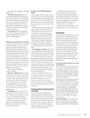
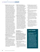
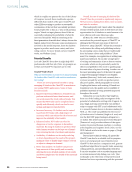
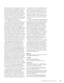
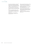
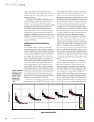
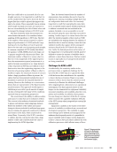
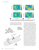
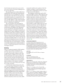
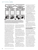
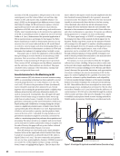
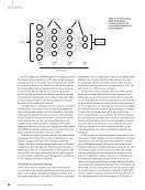
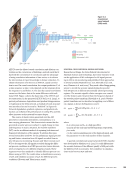
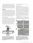
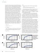
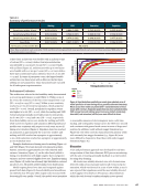
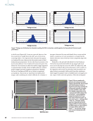
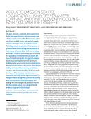
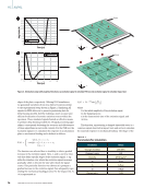
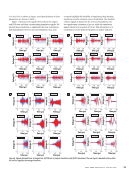
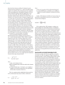
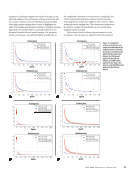
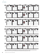
AETCN uses the dilated causal convolution and dilation con- volution as the cornerstone of building a network such that it has both the convenience of convolution and the advantage of using correlation information of time series, so it reduces the intervention of expert knowledge in feature extraction. To obtain information over time in an AETCN, causal convolu- tion is used. In causal convolution, the output prediction Yt of a time sequence at time t only depends on the timesteps from the sequence Xt and before Xt. The fact that causal convolution cannot see the future data is the main difference with tradi- tional CNN. Figure 4 shows the basic idea of the AETCN and its construction. In the proposed AETCN by Li et al. (2022), to prevent performance degradation and gradient disappearance or explosion in the deep network, a residual network structure was introduced as can be seen by “Resblock” in Figure 4b. Network degradation, gradient explosion, and gradient sub- traction can influence the performance of a deep NN, and this effect increases as the network becomes deeper. The source of elastic waves generated over the AM processes is commonly intermittent, nonstationary, or a time-varying phenomena. This characteristic means that the generated acoustic waves are subject to rapid change in time and frequency. In such a situation, the wavelet transform (WT) can be an efficient method of capturing both time and frequency information of the signals. To address this issue, several researchers used WT for the preliminary signal process- ing and feature extraction from AE signals recorded from in situ AM process monitoring. Hossain and Taheri (2021a) used WT to decompose the AE signals recorded during the differ- ent process conditions in a DED process into various discrete series of sequences over different frequency bands. These segments were then analyzed to identify different process con- ditions using a CNN. The results show a classification accuracy of 96% and validation accuracy of 95% for different process conditions (Hossain and Taheri 2021a, 2021b). SPECTRAL CONVOLUTIONAL NEURAL NETWORK Researchers at Empa, the Swiss Federal Laboratories for Materials Science and Technology, have done extensive work on the application of ML techniques for AE signal process- ing in AM in situ monitoring and published their approaches in several articles (Masinelli et al. 2021 Shevchik et al. 2018, 2019 Wasmer et al. 2018, 2019). They used a fiber Bragg grating sensor to record the acoustic signals during the powder bed AM process at different intentionally altered processing regimes. The acoustic signals’ relative energies were consid- ered the features and extracted from the frequency bands of the wavelet packet transform (Shevchik et al. 2018). Wavelet packet transform can be described as applying a set of filters on a signal, as shown by Equations 1 and 2: ​ ​ (1)​ ​ φ​j​​​(n)​ =​ ∑ n​ ​ ​ h0​​​(k)​√M​ ​ ​ _φ(Mn ​ − k)​, k ⊂ Z​​ ​ ​ ​ (2)​ ψ​ji​​​(n)​ =​ ∑ n​ ​ ​ hm−1​​​(k)​√M​ ​ ​ _ψ(Mn ​ − k)​, k ⊂ Z​​ where ​ ​ h​0​​​ is a low pass and ​​ ​ m​​​ is a high pass filter, φ and ψ are the scale and wavelet functions, respectively, j is a scale, n is the current sampling point of the digitized signal, and the parameter m is the total number of filter channels. A spectral convolutional neural network (SCNN) classifier was developed by Mathieu et al. (2014). It could differentiate the acoustic features of the different quality of AM parts with the different level of porosities. The confidence in classifica- tions varies between 83% and 89%. Conv-1 Conv-2 Conv-3 Conv-4 FC-6 FC-7 56 × 56 × 256 28 × 28 × 512 14 × 14 × 512 7 × 7 × 512 1 × 1 × 4096 1 × 1 × 1000 224 × 224 × 64 FC-8 Conv-5 Convolution +ReLU Max pooling Fully connected +ReLU 112 × 112 × 128 Figure 3. A convolutional neural network (CNN) model. J U L Y 2 0 2 3 • M A T E R I A L S E V A L U A T I O N 55 2307 ME July dup.indd 55 6/19/23 3:41 PM SOURCE: LEARNOPENCV (2023)

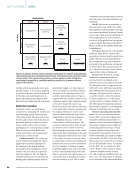
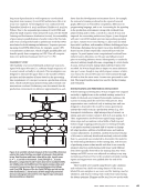
REINFORCEMENT LEARNING Using the same dataset, the Empa group studied the appli- cation of a reinforcement learning (RL) approach to classify different levels of quality for parts manufactured using AM (Wasmer et al. 2019). The RL technique is inspired by the human cognitive capabilities of learning in its surrounding world. In RL, knowledge is acquired through trial and error (or reward and penalty) in an environment by performing the actions and seeing the results of actions (Sutton and Barto 2018). In their approach, a Markovian process is the way of interaction between the RL agent and the environment. The initial state was set to ​​ ​ 0​​​ in the classification process and the algorithm reached the goal ​​ ​ g​​​ by the actions that win the maximum reward. The governing equation for the optimal reward is given by Equation 3: ​ ​ (3)​ ​​ ​​ ​​ ​​ ​ Tπ​​​(s)​ ​ =E​ {​ ∑ t​ ​ λR(​s​t​​, ​ π[​s​t​​]​)​​|​​​s​0​​ ​ =s​ }​ ​ where E is the expectation, the discount factor λ ⊂ [0,1), and π(st) is a policy that maps the states to the actions, and R is the space of the rewards. ME |AI/ML Padding unit Input layer Hidden layer Output layer Y t –2 d =8 d =4 d =2 d =1 Y t –1 Y t X t –2 X1 X2 X3 … … X t –1 X t Detail construction of Resblocks Previous Resblock Resblock Output Softmax Fully connected Resblock Resblock Resblock Input AE signals 9 Resblocks Skip connection 8 4 2 Dilation rate Drop out ReLU Weight norm Dilated causal convolution Drop out ReLU Weight norm Dilated causal convolution 1D convolution Next Resblock Figure 4. Acoustic emission temporal convolution network: (a) basic concept (b) construction (Li et al. 2022). 56 M A T E R I A L S E V A L U A T I O N • J U L Y 2 0 2 3 2307 ME July dup.indd 56 6/19/23 3:41 PM …