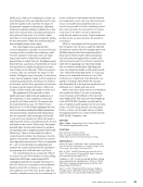
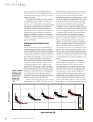
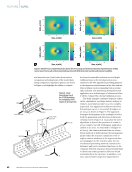
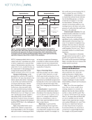
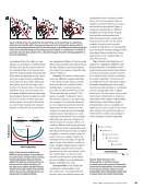
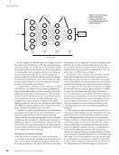
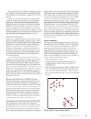
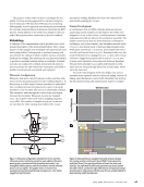
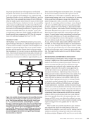
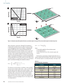
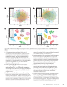
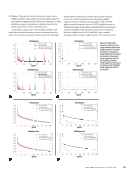
introduced material contaminations in Ramalho et al.’s work, and acoustic signals were recorded during the manufacturing process. Power spectral density (PSD) and short time Fourier transform (STFT) were used to pinpoint the location of dis- continuity formation (Ramalho et al. 2022). Active acoustic methods, or ultrasonic, have also been studied for in situ mon- itoring of the WAAM process. Hossain et al. (2020) designed a fixture to connect an ultrasonic transducer to the build plate of the WAAM system and keep it in constant contact during the manufacturing process. The features extracted from ultrasonic signals showed that there is a detectable difference between the values of root mean square (RMS), root-sum-of-square (RSSQ), and peak magnitude-to-RMS ratio (P2R), which was interpreted as the indication in process deviation from the typical window of WAAM (Hossain et al. 2020). The features extracted from AE signals can be correlated with the AM process condition through statistical signal processing and ML techniques or be used to identify the potential discontinuities in the manufactured parts. Despite the large amount of infor- mation that can be extracted from AE signals, challenges exist in interpreting the signals due to the potentially low signal-to- noise ratio (SNR) and significant variation in the magnitude or frequency of the AE signal over the monitoring period of the AM process. The literature discussed previously reveals that AE shows a promising ability to distinguish variations in the oper- ating conditions of AM systems, known as process conditions. The contrast between AM process conditions is the main cause of quality variation and changes in AM parts. Studies have also shown that AE not only distinguishes between contrary AM processing conditions, which potentially cause different types of defects, but also differentiates various levels of defects. As an example, Shevchik et al. (2019) showed that three levels of quality categories of AM parts manufactured by LPBF can be identified by detecting AE signals analyzed by ML techniques. In their study, quality categories are defined as high, medium, and poor corresponding to various levels of porosity of 0.07%, 0.30%, and 1.42%, respectively (Shevchik et al. 2019). Machine Learning Techniques for Acoustic Data Processing Massive datasets are ubiquitous across scientific and engi- neering disciplines in the current era, and this trend can be attributed to the meteoric rise in computing power over the past few decades. Consequently, applying ML algorithms to infer patterns and gain insight from these datasets has become a new mode of scientific inquiry (Brunton et al. 2020). The NDT industry is no exception to this trend, especially for AET. ML is a subset of AI and is usually divided into three main categories: supervised, unsupervised, and reinforcement learning. Several learning algorithms fall under each of these categories, and in the context of NDT, the fundamental task is to discover or find discontinuities in the specimen of interest. This section aims to avoid discussing ML jargon for brevity. Instead, this paper will elucidate the workings of selected ML algorithms relevant to AE testing as applied to AM. This paper will explain mathematical concepts with analogies, where nec- essary, to reach a wider audience. One of the challenges in AE signal processing is the high level of dependency on human expert participation. However, this could be a major limiting factor when AE is used for in situ monitoring and control of the manufacturing processes. Specifically, this can be an issue when instant and accurate feedback is desired. AE is a data-intensive technology and using ML algorithms to analyze large datasets is of consider- able interest to researchers and practitioners. Additionally, uti- lizing ML algorithms makes the technique more quantitative and less vulnerable to subjective judgments made by techni- cians and engineers when analyzing AE test data. However, despite the large amount of information that can be extracted from AE signals, challenges exist in interpreting the signals due to the potentially low SNR and a considerable variation in the magnitude or frequency of an AE signal over the monitoring period of the AM process. The forthcoming sections briefly discuss how classifiers using various ML techniques are built to help sort AE data obtained from AE systems in the context of AM. ML methods can handle these situations with reasonable efficiency. However, there are still some challenges associated with various ML techniques that must be resolved. Supervised Classification of AM Process States Supervised learning refers to a learning paradigm that requires prior knowledge of the answers to the problem at hand, which implies providing both the input data and the correspond- ing output labels when training the ML model. The model then learns a pattern to better predict or classify future data based on the knowledge from the examples during training. Supervised learning is analogous to a pupil learning a subject by studying a set of questions and their corresponding answers. Classes of problems that require supervised learning include regression and classification problems. Neural Networks This section provides an overview of neural networks, includ- ing the differences between artificial neural networks (ANNs), convolutional neural networks (CNNs), spectral convolutional neural networks (SCNNs), reinforcement learning (RL), and support vector machines (SVMs). ARTIFICIAL NEURAL NETWORKS ANNs are a commonly utilized ML architecture, modeled loosely on the human brain, mimicking how biological neurons communicate with one another. The perceptron, demonstrated by Frank Rosenblatt of Cornell in 1958, was the first trainable neural network (NN) (Rosenblatt 1958). However, it consisted of only a single layer, as opposed to the modern iteration of neural nets (also known as feedforward NNs), which have multiple layers of neurons (multilayer percep- tron, or MLP). Figure 2 shows a sample ANN with one input layer (with five neurons), two hidden layers (each with four neurons), and one output layer with two neurons. J U L Y 2 0 2 3 • M A T E R I A L S E V A L U A T I O N 53 2307 ME July dup.indd 53 6/19/23 3:41 PM

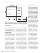
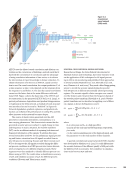
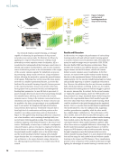
In NNs, weights are coefficients that act as scaling factors for the output of any given layer in an NN. They are the fundamen- tal parameters of an NN, and the aim is to optimize the values of these scalars to minimize the objective (or loss) function during the training phase. Back propagation (also known as backprop for short) is the primary algorithm for performing gradient descent on NNs. It involves performing a forward pass through the network by computing the output value of each node. Then, a backward pass through the network is performed, adjusting the values of the weights in the network. A weighted linear combination of all its inputs is calculated at each neuron. The inputs to the neurons are multiplied by their corresponding weights and then summed up. The result is then passed through an activation function. The activation function decides if the neuron should be activated or not and, if activated, decides its value. The sigmoid function is one example of an activation function. Training an NN requires defining the objective or loss function, typically the mean squared error (MSE) for regression problems or the cross-entropy loss for binary classification problems (relevant to NDT). With the rise of more powerful hardware, especially graphics processing units (GPUs), NNs can now be trained faster, requir- ing less computational hours while simultaneously being “deeper.” The “deep” in deep learning simply refers to the depth of layers in an NN, typically in the hundreds and thousands of hidden layers. The use of deep NNs has revolutionized the field of AI and ML, and frameworks such as PyTorch allow engineers in various fields to apply these powerful algorithms to problems in their respective domains of expertise. CONVOLUTIONAL NEURAL NETWORK CNNs, also known as ConvNets, are a class of NNs that are exceptionally well-suited for applications involving images and videos, such as image and video recognition, driverless cars, and image classification. Like ANNs, CNNs have an input layer, hidden layers, and an output layer. However, the hidden layers will have one or more convolution layers (hence the name). In conjunction with the convolution layers, CNNs also have pooling layers, and together form a single layer of a CNN. The architecture of a CNN is shown in Figure 3. The function of the convolution layer is to detect specific features in an image using the convolution operation that utilizes the concept of the inner (or dot) product between two vectors. In a CNN, the convolution operation is executed using a kernel that is the same size as the window of data it operates on. It is important to note that the kernel elements are weights the network learns when trained. The pooling layer is utilized to reduce the spatial dimension of the data, which helps reduce computational costs and makes the network resistant to overfitting. Each convolution layer has a rectified linear unit (ReLU) activation function that converts all negative values to zeros. The fully connected layer is not a characteristic of the CNN and contains an activation function just like an ANN, converting features into class probabilities (in classification problems). CNNs can process data with a similar grid structure. Local connections, weight sharing, and down-sampling are the main characteristics of CNNs that make them suitable for several types of AE signal analysis. CNN methods are based on the translation invariance of feature extraction and ignore the time correlation of signals. In the case of cyclic NNs, the complex structure and numerous parameters involved in the process make them difficult to optimize and train. Considering these limitations and challenges, research needs to be done to enhance the application of deep learning techniques for AE in situ monitoring for manufacturing processes, specifically in the case of AM. Li et al. (2022) presented a new AE signal recogni- tion method based on a temporal convolution network called acoustic emission temporal convolution network (AETCN) for real-time polymer flow state monitoring in an FDM process. ME |AI/ML Figure 2. An artificial neural network with various components labeled. The arrow shows the direction of back propagation. Weights Neurons Input size Back propagation Input layer Hidden layer 1 Hidden layer 2 Output layer Output size 54 M A T E R I A L S E V A L U A T I O N • J U L Y 2 0 2 3 2307 ME July dup.indd 54 6/19/23 3:41 PM