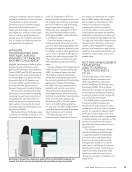
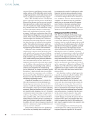
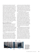
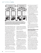
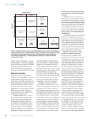
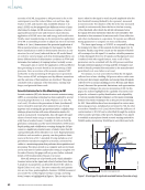
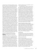
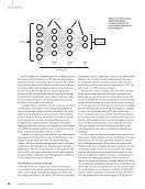
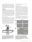
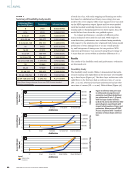
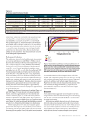
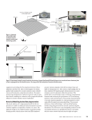
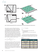
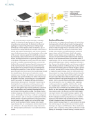
equipment and settings for this experiment mirrored those utilized for the PLB tests. The recorded signals were distin- guished and examined for acoustic emission source identifi- cation and localization, using these procedures. The experi- mental setup facilitated the collection of precise and accurate data, thereby enabling the evaluation of the proposed method’s efficacy in acoustic emission source localization. Numerical Modeling Assisted Data Augmentation This study utilizes a 3D computational model for the test specimen to enable an enhanced characterization of acoustic emission impulses, as inspired by Cuadra et al. (2015). The approach hinges on the implementation of pretrained deep learning models, which harness data from FEM-simulated acoustic emission impulses derived from impact-type and PLB tests (Hamstad 2007). The creation of pretraining data via these simulated AE signals propels advancements in acoustic emission source localization within the specimen. This model offers several benefits, such as reducing computational demands and enhancing the performance of AE monitoring systems in real-world scenarios. The accurate characterization of acoustic emission impulses is a vital prerequisite for devel- oping effective signal-processing algorithms. Our proposal presents a robust methodology to pretrain deep learning models using data procured from acoustic emission impulse simulations. The PLB source was strategically positioned in the out-of-plane direction at a predefined location on the plate, with the sensor situated an inch from the right and upper FO sensor is flexibly mounted to the sample surface AE source FBG-FPI sensor Laser source Circulator Laser Polarization controller DC1 AC1 Photodetector Phase modulator LPF (25 kHz) Amp 40 dB BPF (50–500 kHz) Oscilloscope z y x Figure 1. Schematic of novel fiber-optic coil-based acoustic emission sensing and monitoring system. Lead Mechanical pencil Specimen Specimen 45º Steel ball Sensor Zone 1 Zone 2 Zone 3 Zone 4 Zone 5 Zone 6 Zone 7 Zone 8 Zone 9 Figure 2. Experimental setup for acoustic emission monitoring: (a) pencil lead break (PLB) and (b) impact tests conducted on an aluminum plate (c) that is segregated into nine identified zones. This setup assists the localization of acoustic emission sources. J U L Y 2 0 2 3 • M A T E R I A L S E V A L U A T I O N 73 2307 ME July dup.indd 73 6/19/23 3:41 PM Oscilloscope/DA

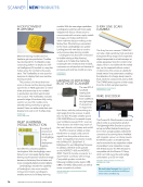
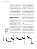
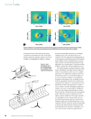
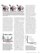
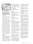
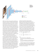
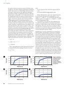
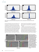
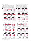
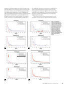
edges of the plate, respectively. Utilizing FEM simulations, we generated waveforms from nine distinct locations similar to the experimental setup shown in Figure 2. Simulating AE signals via FEM allows us to generate pretraining data for deep learning models, thereby enabling a more accurate and efficient localization of acoustic emission sources within the specimen. These simulated signals furnish an effective means to pretrain deep learning models for AE signal processing algo- rithms, consequently bolstering the accuracy and effectiveness of these algorithms in real-world contexts. For the PLB test, the excitation signal, ​​ ​ 1​​​(t)​​ simulates the response of an aluminum plate to mechanical loading and is defined as follows: ​ ​ F1​​​(t)​ ​ =​ {​ − 2t/​t​1​​, 0 x ​ t1​​​ ​ − cos​ π[t ​ − ​ t​1​​]​)​ − 1, ​ t​1​​ x ​ t​2​​​ 0,​t​2​​ x ​ ​ ​ The function was selected due to its ability to elicit a gradual increase in the excitation signal. Here, ​​ ​ 1​​​ and ​​ ​ 2​​​ are time inter- vals that define specific stages of the excitation signal. ​​ ​ 1​​​ sig- nifies the duration over which the excitation signal increases gradually, while ​​ ​ 2​​​ denotes the time after which the signal ceases. This particular function was chosen as it prompts a gradual increase in the excitation signal, thus adequately repre- senting the mechanical loading process. For the impact test, ​​ ​ 2​​​ (t)​​ is represented as: ​ ​ F​2​​​(t)​ =C ​ e​​ −γt/​t​0​​​ sin​ (​ 4π _1 +​​ t​0​​ t ​ ​ ​​ where C is the initial amplitude of the excitation signal, γ is the damping factor, ​ ​ t​0​​​ is the characteristic time of the excitation signal, and t is time. This function, representing a damped sinusoidal wave, is a common signal observed in impact tests and serves to simulate the material response to mechanical loading. The shape of the ​ ​ 0 –0.2 –0.4 –0.6 –0.8 –1 –1.2 –1.4 –1.6 –1.8 –2 0.8 0.6 0.4 0.2 0 –0.2 –0.4 0 2 4 6 8 10 Time (μs) 0 2 4 6 8 10 Time (μs) z y x z y x Sensor 12 in. 12 in. Sensor Zone 1 Zone 4 Zone 5 Zone 6 Zone 9 Zone 8 Zone 7 Zone 2 Zone 3 Zone 1 Zone 4 Zone 5 Zone 6 Zone 9 Zone 8 Zone 7 Zone 2 Zone 3 Ramp function Impact source Figure 3. Simulation setup with analytical functions: (a) excitation signal to simulate PLB test (b) excitation signal to simulate impact test. T A B L E 1 Parameters for simulation Parameters Values Young’s modulus 206 GPa Poisson’s ratio 0.3 Density 2710 kg/m3 t0 5 μs t1 6.5 μs t2 7.5 μs Decay rate γ 1.85 ME |AI/ML 74 M A T E R I A L S E V A L U A T I O N • J U L Y 2 0 2 3 2307 ME July dup.indd 74 6/19/23 3:41 PM Amplitude (N) Amplitude (N)