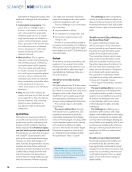
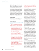
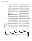
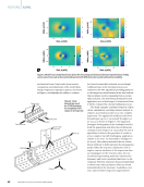
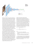
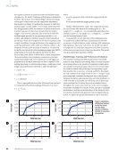
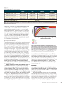
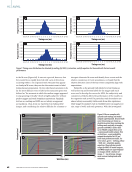
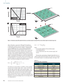
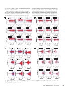
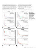
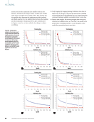
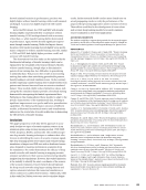
F1(t) and F2(t) shown in Figure 3 and specifications of these parameters are shown in Table 1. Figure 4 showcases the signals derived from the impact and PLB tests and their corresponding simulation signals. We present these waveforms to emphasize the clear correlations and dissimilarities between test and simulation data such contrasts highlight the feasibility of employing deep learning models in acoustic emission source localization. The duration of these signals is distinct for the tests and simulations the test signals span a duration of 250 μs, while the simulation signals extend over a period of 100 μs. This discrepancy is a consequence of the methods employed to gather sufficient Location 2 Location 3 Location 4 Location 5 Location 6 Location 7 Location 8 Location 9 4 2 0 –2 –4 0 100 200 Time (μs) 4 2 0 –2 –4 0 100 200 Time (μs) 2 0 –2 –4 0 100 200 Time (μs) 2 0 –2 –4 0 100 200 Time (μs) 4 2 0 –2 –4 0 100 200 Time (μs) 4 2 0 –2 –4 0 100 200 Time (μs) 4 2 0 –2 –4 0 100 200 Time (μs) 4 2 0 –2 –4 0 50 100 Time (μs) 4 2 0 –2 –4 0 50 100 Time (μs) 4 2 0 –2 –4 0 50 100 Time (μs) 4 2 0 –2 –4 0 50 100 Time (μs) 4 2 0 –2 –4 0 50 100 Time (μs) 4 2 0 –2 –4 0 100 200 Time (μs) 4 2 0 –2 –4 0 100 200 Time (μs) 5 0 –5 0 50 100 Time (μs) 5 0 –5 0 100 200 Time (μs) 5 0 –5 0 100 200 Time (μs) 5 0 –5 0 100 200 Time (μs) 5 0 –5 0 100 200 Time (μs) 5 0 –5 0 100 200 Time (μs) 5 0 –5 0 100 200 Time (μs) 5 0 –5 0 100 200 Time (μs) 5 0 –5 0 100 200 Time (μs) 5 0 –5 0 100 200 Time (μs) 5 0 –5 0 50 100 Time (μs) 5 0 –5 0 50 100 Time (μs) 5 0 –5 0 50 100 Time (μs) 5 0 –5 0 50 100 Time (μs) 5 0 –5 0 50 100 Time (μs) 5 0 –5 0 50 100 Time (μs) 5 0 –5 0 50 100 Time (μs) 5 0 –5 0 50 100 Time (μs) 5 0 –5 0 50 100 Time (μs) 6 4 2 0 –2 –4 0 50 100 Time (μs) 6 4 2 0 –2 –4 0 50 100 Time (μs) 6 4 2 0 –2 –4 0 50 100 Time (μs) Location 1 Location 2 Location 3 Location 4 Location 5 Location 6 Location 7 Location 8 Location 9 Location 1 Location 2 Location 3 Location 4 Location 5 Location 6 Location 7 Location 8 Location 9 Location 1 Location 2 Location 3 Location 4 Location 5 Location 6 Location 7 Location 8 Location 9 Location 1 Figure 4. Signals obtained from: (a) impact test (b) PLB test (c) impact simulation and (d) PLB simulation. The raw signal is denoted in blue, while the red line signifies the average waveform. J U L Y 2 0 2 3 • M A T E R I A L S E V A L U A T I O N 75 2307 ME July dup.indd 75 6/19/23 3:41 PM Voltage (V) Voltage (V) Voltage (V) Voltage (V) Voltage(V) Voltage(V) Voltage(V) Voltage (V) Voltage (V) Voltage (V) Voltage (V) Voltage (V) Voltage(V) Voltage(V) Voltage (V) Voltage(V) Voltage (V) Voltage (V) Voltage (V) Voltage (V) Voltage (V) Voltage (V) Voltage(V) Voltage(V) Voltage (V) Voltage (V) Voltage (V) Voltage (V) Voltage(V) Voltage(V) Voltage(V) Voltage (V) Voltage (V) Voltage (V) Voltage (V) Voltage (V)

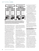
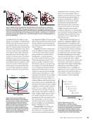
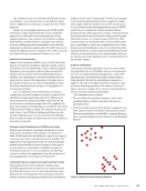
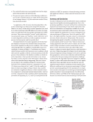
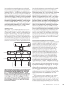
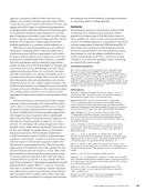
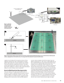
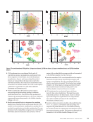
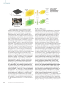
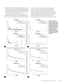
data from finite element modeling. We deployed a point domain network consisting of a 5 × 5 grid of sensing locations to gather the simulation data, which increases the complexity of the surrounding mesh, substantially slowing the collection of the reverberation pattern (reflected signals after 100 μs). As such, for practicality and computational efficiency, we limited the simulation data collection to the initial 100 μs. The simulation was conducted using a workstation equipped with a 3.1 GHz multi-core processor and a 4 GB dedicated graphics card. On average, each round consumed approximately 40 min. To gather an adequate volume of source domain data (simulation dataset), a data augmentation process was executed, resulting in the accumulation of 900 waveforms. It is noteworthy that differences in the reflection and trigger mechanisms between simulations and experiments, as observ- able in the figures, stem from variations in the interaction with adjacent substrates and boundary conditions, resulting in distinct reverberation patterns. Furthermore, while the simula- tion model logs the accurate time of arrival, the experimental process depends on manual trigger thresholding. t-SNE is a powerful technique for visualizing high-dimensional data by mapping each data point to a two- or three-dimensional space. While t-SNE was originally designed for static data, it has been adapted for use with time series data in some cases. Visualizing AE data can be challenging due to its complexity and high dimensionality. However, t-SNE can be used to map time series data onto a low-dimensional space while preserving its underlying structure. To apply t-SNE to time series data, we first need to transform the sequential nature of the data into a set of fixed- length feature vectors that can be used as input to t-SNE. This can be done using various techniques such as sliding windows or feature extraction methods like Fourier transforms or wavelet transforms. Once we have transformed the time series data into feature vectors, we can compute pairwise similarities between them using a Gaussian kernel: pI,j = exp( − |xi – xj|| 2 _2 σ 2 ) ________________ ∑ k ∑ l exp(−_) ||xk – xl|| 2 2 σ 2 where xi and xj are two feature vectors, sigma is a parameter that controls the width of the Gaussian kernel, and pI,j is the probability that xi would pick xj as its neighbor if neighbors were picked in proportion to their probability density under a Gaussian centered at i .Next, we compute pairwise similarities between points in the low-dimensional map using a Student-t distribution: qi,j = (1 + |yi − yj|| 2 ) −1 __________________ ∑ k ∑ l (1 +||yk − yl|| 2 ) −1 where yi and j are two points in the low-dimensional map, and qi,j is the probability that yi would pick j as its neighbor if neighbors were picked uniformly at random from all other points. Finally, t-SNE minimizes the difference between these two distributions using gradient descent on a cost function that measures their divergence: KL(P‖Q) = ∑ i ∑ j pi,jlog pi,j qi,j We’ve employed this t-SNE technique to enhance our understanding of the relationship between our simulation and experimental datasets. Two-dimensional plots generated by this method, as depicted in Figure 5, showing the similar- ities between AE signals collected from nine distinct zones. Figures 5a and 5b demonstrate that the experimental data from both the impact and PLB tests exhibit larger variability and less distinct clustering, suggesting more complexities and uncer- tainties in real-world scenarios. On the other hand, Figures 5c and 5d illustrate that the simulation data from both tests have a clearer clustering effect, indicating the advantages of using controlled and predictable simulation data for improving AE source localization techniques. Nevertheless, it’s important to recall that the simulation data might not encapsulate all the complexities and variations inherent in real-world scenarios. Therefore, further optimization of our proposed source local- ization techniques is necessary to incorporate more uncer- tainty factors, ensuring effectiveness across diverse real-world applications. Deep Transfer Learning for Knowledge Transfer This study investigates the effective application of transfer learning to new data, leveraging the insights obtained from pretrained models. A variety of deep learning models, includ- ing convolutional neural network (CNN), fully connected neural network (FCNN), Encoder, Residual Network (ResNet), Inception, and Multi-Layer Perceptron (MLP), were assessed for their ability to analyze simulated datasets and to extract underlying features using a layer-wise fine-tuning strategy. The employed methodology entailed signal acquisition from the simulated datasets, followed by data preprocessing, feature extraction via fine-tuned deep learning models, and finally classification based on acoustic emission source location. To scrutinize impact and PLB test simulations, six deep learning models with distinct architectures and capabilities were inves- tigated. This innovative strategy leads to a broader compre- hension of the data, permitting the recognition of overlooked patterns and features when using a singular model. Detailed summaries of the architectures used for the networks men- tioned are as follows: ME |AI/ML 76 M A T E R I A L S E V A L U A T I O N • J U L Y 2 0 2 3 2307 ME July dup.indd 76 6/19/23 3:41 PM
ASNT grants non-exclusive, non-transferable license of this material to  .
All rights reserved. © ASNT 2026. To report unauthorized use, contact: customersupport@asnt.org