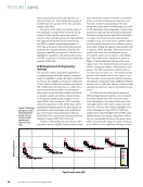
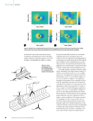
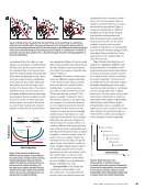
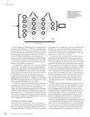
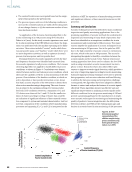
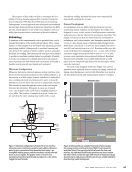
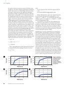
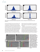
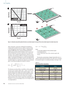
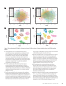
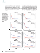
Ñ CNN implements two convolutional blocks with 1D convolutions, instance normalization, and dropout. Each block comprises a Conv1D layer, succeeded by instance normalization, dropout, and max pooling. Hierarchical features are extracted from the input time series by the convolutional blocks. These features are then flattened and transmitted to a SoftMax classifier. The CNN model employs “categorical_crossentropy” loss and Adam optimizer (Simonyan and Zisserman 2014). Ñ FCNN resembles the CNN architecture but replaces max pooling with global average pooling to minimize spatial information loss. The global average pooling layer compacts the spatial information into a 1D vector, with these compressed features then passed to the SoftMax classifier (Zhang et al. 2017). Ñ ResNet uses residual blocks to circumvent the vanishing gradient issue. Residual blocks add the input directly to the stacked convolutional layers, enabling direct gradient flow. It uses batch normalization and weight regularization (L2 regu- larization). Each residual block comprises two Conv1D layers followed by batch normalization and activation, with the output of the residual blocks average pooled and transmitted to the SoftMax classifier size (He et al. 2015). Ñ Encoder resembles CNN’s convolutional blocks but employs Parametric Rectified Linear Unit (PReLU) activation and instance normalization. After the convolutional blocks, an attention mechanism is applied. This attention layer assigns weights to the feature maps, focusing on pertinent features. The attended features are flattened and passed to the SoftMax classifier extraction (Vincent et al. 2008). Ñ MLP substitutes the convolutional layers with dense layers for time series classification. The input time series is flattened and sent to the dense layers. It uses two dense layers with dropout for regularization. The output dense layer utilizes SoftMax activation for the classification (Delashmit and Manry 2005). Ñ Inception utilizes an inception module with parallel branches of 1 × 1, 3 × 3, and 5 × 5 convolutions and max pooling. The outputs of the parallel branches are concatenated, forming the inception module. It employs batch normalization and the dropout post inception module. The features are flattened and transmitted to the SoftMax classifier (Zhang et al. 2022). Zone 1 Zone 2 Zone 3 Zone 4 Zone 5 Zone 6 Zone 7 Zone 8 Zone 9 10 5 0 –5 –10 –15 –10 –5 0 5 10 x-tsne 15 10 5 0 –5 –10 –15 –10 –5 0 5 10 15 x-tsne Zone 1 Zone 2 Zone 3 Zone 4 Zone 5 Zone 6 Zone 7 Zone 8 Zone 9 15 10 5 0 –5 –10 –15 –15 –10 –5 0 5 10 15 x-tsne Zone 1 Zone 2 Zone 3 Zone 4 Zone 5 Zone 6 Zone 7 Zone 8 Zone 9 10 5 0 –5 –10 –15 –15 –10 –5 0 5 10 x-tsne Zone 1 Zone 2 Zone 3 Zone 4 Zone 5 Zone 6 Zone 7 Zone 8 Zone 9 Figure 5. The two-dimensional t-SNE plot for: (a) impact test dataset (b) PLB test dataset (c) impact simulation dataset and (d) PLB simulation dataset. J U L Y 2 0 2 3 • M A T E R I A L S E V A L U A T I O N 77 2307 ME July dup.indd 77 6/19/23 3:41 PM y-tsne y-tsne y-tsne y-tsne

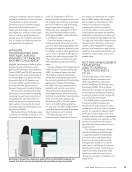
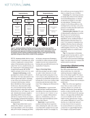
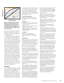
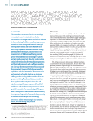
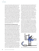
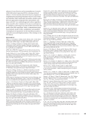
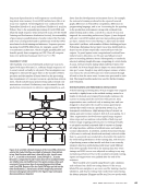
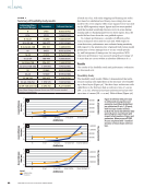
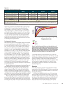
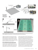
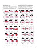
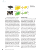
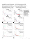
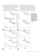
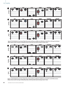
Our research employs transfer learning, a technique capable of enhancing the performance of deep neural networks across various tasks. We illustrate its efficacy by applying it to improve the performance of deep neural networks in acoustic emission source localization. AE is a nondestructive testing method that leverages sound waves to identify and analyze material defects, and acoustic emission source localization pertains to the determination of the origin of the acoustic emission signals. We initialized our process by pretraining a deep neural network on a large simulation dataset, allowing the network to capture the general features of AE signals. Following this, we fine-tuned the deep neural network on a smaller experimental dataset, a process that facilitated the network’s learning of specific features present in the experimental data. Our process involves first trans- ferring layers from a pretrained model, and subsequently freezing their parameters. As new AE data is processed, it passes through these frozen layers before progressing through the trainable layers, allowing us to localize the acoustic emission source. Owing to the intrinsic connection between simulation and experimental data, the feature extractor can be applied to the latter, incorporating it as a nonadjustable layer in our model. We designate the high-level features extracted from these layers as “bottleneck” features due to their high level of condensation and their position at the classifiers’ preceding constriction point (as illustrated in Figure 6). The applied deep learning architecture comprises one of six classifiers, each consisting of multiple fully con- nected layers following global pooling. This design enables nonlinear mapping of bottleneck features to AE source local- ization. Additionally, a fusion layer is utilized to amalgamate extracted features, and an extra layer is employed to link bot- tleneck features to location predictions. During fine-tuning, the pretrained model’s weights serve as the initial values, and the model undergoes further training with available target domain data. As a consequence, the fine-tuned model can acclimatize to the target domain’s unique characteris- tics, offering superior performance to a model trained from scratch. Results and Discussion In this section, we compare the performance of various deep learning models with and without transfer learning applied to acoustic emission source localization tasks. We analyze the mean loss and loss range over 200 epochs for CNN, FCNN, Encoder, ResNet, MLP, and Inception architectures. These models were trained on two different datasets, namely the impact dataset and the PLB dataset, which both contain distinct acoustic emission source localizations. In the first scenario, we trained CNN models without transfer learning directly on the experimental dataset. Both models exhibit a similar pattern over the epochs, initially having high loss values and gradually improving to achieve a significant reduction in loss. However, the validation loss does not decrease as substan- tially, which may indicate overfitting. In this case, the models have learned the training data too well but struggle to general- ize on new, unseen data. In contrast, for the second scenario, we employed transfer learning, where the CNN models were first pretrained on a large, simulated dataset before being fine- tuned on the experimental dataset. Both models begin with lower loss values than those without transfer learning, which could be attributed to the initial learning from the simulated dataset. Over 200 epochs, these models improve significantly. One model achieves a very low validation loss, suggesting excellent generalization capability, while the other model has a slightly higher validation loss. The performance of the other models, such as FCNN, Encoder, MLP, Inception, and ResNet, are also compared with and without transfer learning. Some models, such as the Encoder and MLP, exhibit signifi- cant improvements when transfer learning is applied, while others show minor or negligible differences. Interestingly, the ResNet model demonstrates good performance on both the impact and PLB datasets, with and without transfer learning, though it experiences more fluctuations in the loss curve without transfer learning. Figures 7, 8, and 9 illustrate the mean loss and loss range for each model with and without transfer learning on the impact and PLB datasets. These visualizations provide a clear comparison of the models’ performances, high- lighting the advantages of transfer learning in various cases. In ME |AI/ML Knowledge transfer Frozen layers Bottleneck features Finite element modeling Experimental setup z y x Pretrained layers Zone 1 Zone 2 Zone 3 Zone 9 Localization Zone 1 Zone 2 Zone 3 Zone 9 Figure 6. Schematic and structure of knowledge transfer via deep transfer learning. 78 M A T E R I A L S E V A L U A T I O N • J U L Y 2 0 2 3 2307 ME July dup.indd 78 6/19/23 3:41 PM