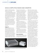
as its magnitude, location, and potential impact on the pipe-
line’s integrity (Liang et al. 2013). The main advantages of using
acoustic signals for gas leak diagnosis include swift response
time, long range, and precise localization (S. Wang and Yao
2020). A key drawback of using acoustic signals is their reduced
sensitivity as the sensors move farther away from the source
due to significant attenuation (Liu et al. 2017). This attenua-
tion is even more pronounced with higher-frequency sounds
(ultrasound), which are often involved with smaller leakages.
One effective approach to mitigate this problem is by employ-
ing an array of microphones along with acoustic imaging
techniques (Li et al. 2021 Fluke 2021 Drives &Controls 2021).
However, this method generates a substantial amount of data,
which is not ideal for a near-real-time approach required for
creating a semi-autonomous platform and quick response.
Fortunately, this issue has been ingeniously addressed by bio-
logical systems in their evolutionary acoustic sensing systems,
using only two ears (binaural sensing). Instead of relying on
increased sensor numbers to enhance sensitivity, these bio-
logical systems evolved their external ear (pinna) shapes to act
as hardware for magnifying sound coming from specific direc-
tions. This evolution was further complemented by strategic
motion and motion control of the pinna and head as well as
their movement (Populin and Yin 1998 Fletcher 2014), allowing
them to dynamically change acoustic directionality and sen-
sitivities as needed. Inspired by these biological mechanisms,
we propose in this paper an acoustic sensing system that com-
prises two microphones, mimicking two ears and binaural
hearing, with a framework designed to optimize or strategize
movement to improve source localization accuracy.
Sound source localization (SSL) is a prominent topic in
robotics, with a detailed review of common methods provided
by Rascon and Meza (2017). While gas and air leak local-
ization is essential for industrial inspections and has been
explored in earlier research, many existing approaches rely on
fixed microphone arrays (Eret and Meskell 2012), handheld
devices (Liao et al. 2013) for manual detection, and statistical
time-domain features for pinpointing leaks in pipes (F. Wang
et al. 2017). Yan et al. (2018) used a four-element linear array to
identify multiple sources with the MUSIC algorithm within the
63–187 kHz emission range. Focusing on ultrasonic emissions
from leaks in pressurized pipes, Schenck, Daems, and Steckel
(2019) employed a peak search on a beam-formed spectrum
and use a 32-element microphone array. By leveraging
multiple poses of the robot and integrating simultaneous local-
ization and mapping (SLAM) techniques with the microphone
array, potential leaks are effectively localized. Most recently,
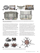
G. K. J. Fischer et al. (2024) introduced an autonomous robotic
system for comprehensive plant inspection, equipped with a
variety of sensors, including lidar, stereo, UV/IR/RGB cameras,
electronic noses, and five microphones. These sensors detect
factors like methane leaks, flow rates, and infrastructure issues.
The system was tested at a wastewater treatment site, achiev-
ing gas leak localization with a 50 cm error through acoustic
assessments.
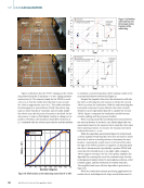
Current robotic systems for industrial inspection rely on
various sensors, such as lidar, stereo, and depth cameras, to
map environments for navigation and distance estimation.
However, little attention has been given to optimizing the
robot’s movement and positioning to enhance leak localiza-
tion once an anomaly, such as sound generated by a leak, is
detected by the microphones. Typically, these systems use
microphone arrays to estimate the direction of arrival (DOA)
of sound, combined with techniques like SLAM and lidar to
locate the leak. While multi-microphone array techniques can
perform well from fixed positions, they often require more
complex hardware setups, increased costs, and larger physical
space. In contrast, the proposed method achieves accurate
localization using a simpler hardware setup (two microphones)
with lower computational demands. This is accomplished by
strategically leveraging the robot’s mobility, effectively trading
hardware complexity and computational power for movement.
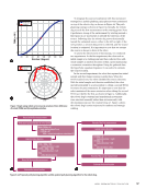
Specifically, this paper explores how motion, combined with
a two-microphone array inspired by an animal’s external
auditory system, enhances sound source localization. In other
words, we focus on optimizing the robot’s movement strat-
egies to acquire samples that enable precise sound source
localization while maintaining a lightweight system configu-
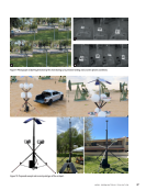
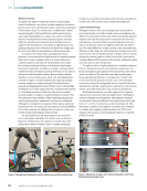
ration. First, we examine the effect of motion using a fixed-
base collaborative robotic arm. Based on the insights gained
from this study, we propose a motion strategy to enhance the
robot’s source localization. Finally, we implement this strategy
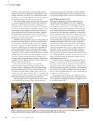
on a quadruped robot to explore its effectiveness for mobile
platforms.
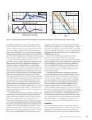
Method
This section provides a comprehensive overview of our meth-
odology, covering the sound source localization approach,
acoustic data acquisition process, robotic systems, and experi-
mental setup.
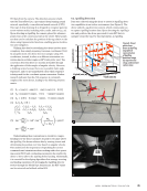
Source Localization Method
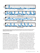
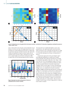
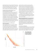
The time difference of arrival (TDOA) between two signals is
commonly estimated by calculating a cross-correlation vector
(CCV). The Pearson correlation factor, as shown in Equation 1,
provides the simplest way of calculating the CCV (Rascon and
Meza 2017):
(1) CCV[τ] =
_ _ Σ________________________)2−]τ________________−_t[2a()1−]t[1a(____________t
√ Σt(a1[t] −
_
1)2 √ Σt(a2[t − τ] −
_
2)2
where
a1 and 2 are the two discrete signals being compared,
τ is the time shift applied to 2 and
_ a1 and a2 _ are the mean values of 1 and 2 respectively.
Although computationally efficient and straightforward,
CCV-based TDOA estimation is highly susceptible to environ-
mental noise and reverberations, often leading to inaccurate
estimates (Brandstein and Silverman 1997). To mitigate these
challenges, the Generalized Cross-Correlation with Phase
ME
|
LEAKLOCALIZATION
52
M AT E R I A L S E V A L U AT I O N • A P R I L 2 0 2 5
line’s integrity (Liang et al. 2013). The main advantages of using
acoustic signals for gas leak diagnosis include swift response
time, long range, and precise localization (S. Wang and Yao
2020). A key drawback of using acoustic signals is their reduced
sensitivity as the sensors move farther away from the source
due to significant attenuation (Liu et al. 2017). This attenua-
tion is even more pronounced with higher-frequency sounds
(ultrasound), which are often involved with smaller leakages.
One effective approach to mitigate this problem is by employ-
ing an array of microphones along with acoustic imaging
techniques (Li et al. 2021 Fluke 2021 Drives &Controls 2021).
However, this method generates a substantial amount of data,
which is not ideal for a near-real-time approach required for
creating a semi-autonomous platform and quick response.
Fortunately, this issue has been ingeniously addressed by bio-
logical systems in their evolutionary acoustic sensing systems,
using only two ears (binaural sensing). Instead of relying on
increased sensor numbers to enhance sensitivity, these bio-
logical systems evolved their external ear (pinna) shapes to act
as hardware for magnifying sound coming from specific direc-
tions. This evolution was further complemented by strategic
motion and motion control of the pinna and head as well as
their movement (Populin and Yin 1998 Fletcher 2014), allowing
them to dynamically change acoustic directionality and sen-
sitivities as needed. Inspired by these biological mechanisms,
we propose in this paper an acoustic sensing system that com-
prises two microphones, mimicking two ears and binaural
hearing, with a framework designed to optimize or strategize
movement to improve source localization accuracy.
Sound source localization (SSL) is a prominent topic in
robotics, with a detailed review of common methods provided
by Rascon and Meza (2017). While gas and air leak local-
ization is essential for industrial inspections and has been
explored in earlier research, many existing approaches rely on
fixed microphone arrays (Eret and Meskell 2012), handheld
devices (Liao et al. 2013) for manual detection, and statistical
time-domain features for pinpointing leaks in pipes (F. Wang
et al. 2017). Yan et al. (2018) used a four-element linear array to
identify multiple sources with the MUSIC algorithm within the
63–187 kHz emission range. Focusing on ultrasonic emissions
from leaks in pressurized pipes, Schenck, Daems, and Steckel
(2019) employed a peak search on a beam-formed spectrum
and use a 32-element microphone array. By leveraging
multiple poses of the robot and integrating simultaneous local-
ization and mapping (SLAM) techniques with the microphone
array, potential leaks are effectively localized. Most recently,
G. K. J. Fischer et al. (2024) introduced an autonomous robotic
system for comprehensive plant inspection, equipped with a
variety of sensors, including lidar, stereo, UV/IR/RGB cameras,
electronic noses, and five microphones. These sensors detect
factors like methane leaks, flow rates, and infrastructure issues.
The system was tested at a wastewater treatment site, achiev-
ing gas leak localization with a 50 cm error through acoustic
assessments.
Current robotic systems for industrial inspection rely on
various sensors, such as lidar, stereo, and depth cameras, to
map environments for navigation and distance estimation.
However, little attention has been given to optimizing the
robot’s movement and positioning to enhance leak localiza-
tion once an anomaly, such as sound generated by a leak, is
detected by the microphones. Typically, these systems use
microphone arrays to estimate the direction of arrival (DOA)
of sound, combined with techniques like SLAM and lidar to
locate the leak. While multi-microphone array techniques can
perform well from fixed positions, they often require more
complex hardware setups, increased costs, and larger physical
space. In contrast, the proposed method achieves accurate
localization using a simpler hardware setup (two microphones)
with lower computational demands. This is accomplished by
strategically leveraging the robot’s mobility, effectively trading
hardware complexity and computational power for movement.
Specifically, this paper explores how motion, combined with
a two-microphone array inspired by an animal’s external
auditory system, enhances sound source localization. In other
words, we focus on optimizing the robot’s movement strat-
egies to acquire samples that enable precise sound source
localization while maintaining a lightweight system configu-
ration. First, we examine the effect of motion using a fixed-
base collaborative robotic arm. Based on the insights gained
from this study, we propose a motion strategy to enhance the
robot’s source localization. Finally, we implement this strategy
on a quadruped robot to explore its effectiveness for mobile
platforms.
Method
This section provides a comprehensive overview of our meth-
odology, covering the sound source localization approach,
acoustic data acquisition process, robotic systems, and experi-
mental setup.
Source Localization Method
The time difference of arrival (TDOA) between two signals is
commonly estimated by calculating a cross-correlation vector
(CCV). The Pearson correlation factor, as shown in Equation 1,
provides the simplest way of calculating the CCV (Rascon and
Meza 2017):
(1) CCV[τ] =
_ _ Σ________________________)2−]τ________________−_t[2a()1−]t[1a(____________t
√ Σt(a1[t] −
_
1)2 √ Σt(a2[t − τ] −
_
2)2
where
a1 and 2 are the two discrete signals being compared,
τ is the time shift applied to 2 and
_ a1 and a2 _ are the mean values of 1 and 2 respectively.
Although computationally efficient and straightforward,
CCV-based TDOA estimation is highly susceptible to environ-
mental noise and reverberations, often leading to inaccurate
estimates (Brandstein and Silverman 1997). To mitigate these
challenges, the Generalized Cross-Correlation with Phase
ME
|
LEAKLOCALIZATION
52
M AT E R I A L S E V A L U AT I O N • A P R I L 2 0 2 5