between the robot controller and the ECA data acquisition
system. The process follows these steps:
1. Normalize each line scan per coil (range: 0 to 1).
2. Compute the mean voltage across all channels at each time
instance.
3. Subtract the mean from the normalized voltages.
4. Convert the normalized values back to the original voltage units.
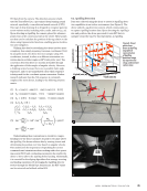
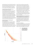
Detrending Algorithms
In addition to array subtraction, three detrending methods are
applied to the ECA data. Detrending is performed across space
using the x and y coordinates, while excluding the z-axis. The
underlying assumption is that robot positioning errors occur at
a lower spatial frequency than corrosion damage, allowing their
removal through detrending. The procedures are as follows:
1. Linear detrending for signals in the time domain.
2. Planar spatial detrending (1​ ​ order) along x and y coordinates.
3. Higher-order spatial detrending (3​ ​ order) along x and y
coordinates.
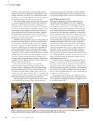
Experimental Validation of Robotic ECA System
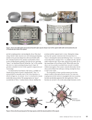
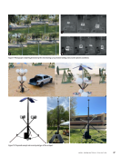
This section presents the experimental validation of the robotic
ECA system on curved steel samples with corrosion damage.
Additionally, we demonstrate the application of the proposed
image processing algorithm for enhanced damage detection.
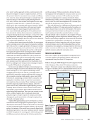
Acquisition and Processing of ECA Measurements
This section presents the experimental ECA measurements
obtained using the developed robotic setup and their com-
parisons with microscopic images of corroded steel samples.
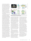
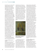
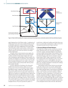
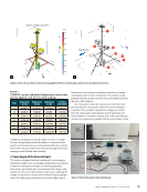
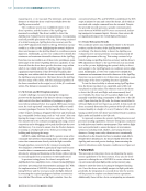
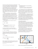
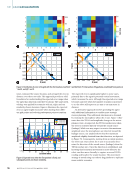
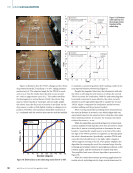
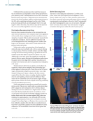
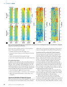
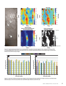
Figure 6 outlines the ECA data processing workflow for flat
Sample A, where all voltage processing is performed along
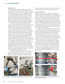
the x and y coordinates. Figure 6a displays raw measure-
ments from individual coils, while Figure 6b illustrates the
scan using the ECA probe. The array subtraction algorithm is
applied to remove common coil trends from the array image
data. The final processed image, shown in Figure 6c, results
from detrending to eliminate liftoff and tilt variations, with the
detrend magnitude detailed in Figure 4b.
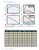
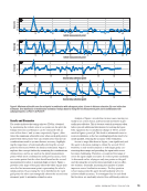
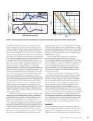
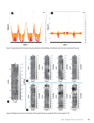
Figure 7 demonstrates the effect of processing ECA data
over time. In Figure 7a, voltage spikes occur as the array probe
nears the sample edge due to increased liftoff. These artifacts
are largely removed in Figure 7b after processing.
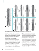
Figures 8 and 9 present the results for both full and
fast scans after the post-processing steps described earlier.
Corrosion is visible in most datasets, though some inaccuracies
persist post-processing. Full scans, acquired using Coil 16 near
the center of the array, exhibit tilting effects along the x-axis in
0.5
0.4
10
5
0
—5
—10
0.3
0.2
0.1
—0.1
—0.2
—0.3
—0.4
—0.5
0
0.5
0.4
0.3
100
50
0 0
–50
–100
0.2
0.1
—0.1
—0.2
—0.3
—0.4
—0.5
0
Absolute real Absolute real
100
100
50
0
—50
—100
100
50
0
—50
—100
100
50
0
—50
—100
100
50
0
—50
—100
100
50
0
—50
—100
100
50
0
—50
—100
100
50
0
—50
—100
100
50
0
—50
—100
50
–50 ...
...
–100
1010 1030
x (mm)
Coil 32 Coil 30
1050 1030 1050
x (mm)
1070 1030 1050
x (mm)
1070
Coil 4 Coil 2
1000 1020
x (mm)
1040 1000 1020
x (mm)
1040
Coil 3 Coil 1
1000 1020
x (mm)
1040 990 1010
x (mm)
1030
Coil 31 Coil 29
1030 1050
x (mm)
1070 1030 1050
x (mm)
1070
1010 1030
x (mm)
1050
Absolute real
Figure 6. Post-processing of ECA image data in spatial domain: (a) raw data per each coil (b) diagnostic image after array subtraction (c) diagnostic
image after array subtraction and detrending.
ME
|
ROBOTICECA
68
M AT E R I A L S E V A L U AT I O N • A P R I L 2 0 2 5
y
(mm)
y
(mm)
R
1
(odds)
Row
2
(evens)
y
(mm)
y
(mm)
V oltage
(V)
V
(V)
V oltage
(V)

1
2
3
4
5
6
7
8
9
10
11
12
13
14
15
16
17
18
19
20
21
22
23
24
25
26
27
28
29
30
31
32
Coilssi 1
2
3
4
5
6
7
8
9
10
11
12
13
14
15
16
17
18
19
20
21
22
23
24
25
26
27
28
29
30
31
32
Coils
5
0
—5
0 5 10 15 20
Time (s)(
25 30 35 40
10
15
20
5
0
—5
0 5 10 15 20
Time (s)
25 30 35 40
10
15
20
i
i e (
—
Figure 7. Post-processing of ECA line scans using array subtraction and detrending in time domain: (a) raw line scans (b) processed line scans.
100
50
0
0
—0.1
—0.2
—0.3
—0.4
—0.5
0.1
0.2
0.3
0.4
0.5
x (mm)
A
1020 1040
—50
—100
100
50
0
0
—0.1
—0.2
—0.3
—0.4
—0.5
0.1
0.2
0.3
0.4
0.5
x (mm)
C1
1020 1040
—50
—100
100
50
0
0
—0.1
—0.2
—0.3
—0.4
—0.5
0.1
0.2
0.3
0.4
0.5
x (mm)
C2
1010 1030 1050
—50
—100
100
50
0
0
—0.1
—0.2
—0.3
—0.4
—0.5
0.1
0.2
0.3
0.4
0.5
x (mm)
C3
1020 1040
—50
—100
100
50
0
0
—0.1
—0.2
—0.3
—0.4
—0.5
0.1
0.2
0.3
0.4
0.5
x (mm)
C4
1010 1030 1050
—50
—100
100
50
0
0
—0.1
—0.2
—0.3
—0.4
—0.5
0.1
0.2
0.3
0.4
0.5
x (mm)
B1
1020 1040
—50
—100
100
50
0 0
—0.1
—0.2
—0.3
—0.4
—0.5
0.1
0.2
0.3
0.4
0.5
x (mm)
B2
—50
—100
100
50
0 0
—0.1
—0.2
—0.3
—0.4
—0.5
0.1
0.2
0.3
0.4
0.5
x (mm)
B3
1020 1040 1020 1040 1020 1040
—50
—100
100
50
0
0
—0.1
—0.2
—0.3
—0.4
—0.5
0.1
0.2
0.3
0.4
0.5
x (mm)
B4
—50
—100
Figure 8. Full eddy current scans for steel samples: (a) flat sample A (b) concave samples B1–B4 (c) convex samples C1–C4.
A P R I L 2 0 2 5 • M AT E R I A L S E V A L U AT I O N 69
V oltage
(V)
Vo ltage
(V)
Vo ltage
(V)
V
(V
)
Vo ltage
(V)
Vo ltage
(V)
Vo ltage
(V)
Vo ltage
(V)
Vo ltage
(V)
Voltagee(V) Voltagee(V)
y
(mm)
y
(mm)
y
(mm)
y
(mm)
y
(mm)
y
(mm)
y
(mm)
y
(mm)
y
(mm)