instructions issued and real-time Cartesian position and ori-
entation data received at a frequency of approximately 70 Hz
through an Ethernet connection. The system integrates three
key sensors: (1) a structured-light (SL) camera, (2) a calibration
laser profilometer, and (3) an eddy current array (ECA).
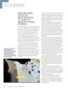
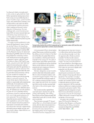
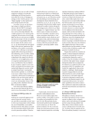
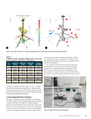
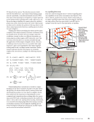
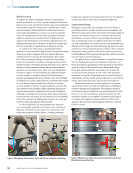
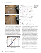
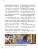
The structured-light camera with a reconstruction accuracy
of 0.1 mm is positioned remotely from the robot as shown in
Figure 2a. It captures the part’s geometry, enabling precise
path planning. The calibration laser profilometer is mounted
in a custom 3D-printed holder, as illustrated in Figure 2b. This
sensor ensures proper alignment between the reconstructed
virtual model and the robot’s physical workspace. Capable of
measuring depths ranging from 50 mm to 150 mm with an
accuracy of 4 µm, the sensor is positioned 60 mm from the cal-
ibration regions of the test specimen.
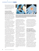
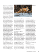
The ECA used in this system is an array of 48 pancake coils
fabricated on a flexible substrate. The ECA is interfaced with
the PC using the multichannel eddy current data acquisition
system via a software development kit (SDK) in C#. Although
the probe is a flexible array, it is mounted on a rigid fixture to
ensure consistent and known coil orientations during opera-
tion. While the probe’s nominal center frequency is 500 kHz, it
is operated at 2 MHz to provide maximum sensitivity to surface
corrosion. The array consists of 48 coils arranged in three rows
of 16, with a 1.25 mm spacing between coils, offering a total
coverage width of 34 mm, as shown in Figure 2c. During data
acquisition, only the right two rows of 16 coils are used, result-
ing in a total of 32 active sensors.
In the system, the ECA supports two operational
modes: impedance (absolute measurements) and reflec-
tion (pitch-catch). A differential mode is also applied during
post-processing using MATLAB. The coils are driven by a 5 V
AC signal, producing complex voltage outputs, with the real
component used for post-processing. The robot is programmed
to position the ECA probe 1 mm above the test surface, though
variations in liftoff can be observed during experiments.
The laser and ECA probe integrated into the robotic setup
are depicted in Figure 2b. Eddy current measurements are
acquired at an update rate of 16 kHz per coil. This configura-
tion provides a spatial resolution of 50 µm along each raster
line, ensuring sufficient detail for effective corrosion detection.
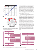
Scan Path Generation for ECA
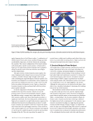
The scan path generation procedure is adapted from the
framework outlined by Hamilton et al. (2024), beginning
with the virtual reconstruction of the scanning environment
using a structured-light camera to create a digital model of
the part. This virtual model is aligned with the physical work-
space through calibration points identified by a laser calibra-
tion sensor. Accurate alignment is ensured by comparing the
physical calibration points in the robot’s workspace with their
virtual counterparts using point-to-point projection. The recon-
structed mesh is further refined by segmenting the sample
from the background and applying decimation and Laplacian
smoothing techniques (Sorkine et al. 2004). A zigzag raster
path is then generated on the refined mesh using a ray-plane
intersection array algorithm (Hamilton et al. 2024), achieving
a point cloud resolution of 0.1 mm × 0.25 mm, which is inter-
polated to 0.2 mm × 0.2 mm for 2D processing. This path is
simulated and converted into robot commands. During the
scanning process, the system PC gathers data streams from the
ECA, alongside real-time orientation data from the robot’s tool
frame. These data streams are processed to ensure accurate
and reliable defect detection.
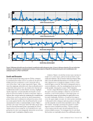
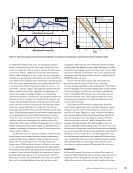
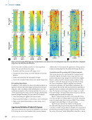
The system utilizes two types of scanning paths. The first,
referred to as a “fast scan,” involves the array coils scanning
the region of interest without redundancy. In this method, the
array probe traverses the test sample only once along its long
side, minimizing scanning time in proportion to the number of
coils in the array. For higher resolution, sub-scans can be per-
formed, where the pathing distance of a coil is smaller than the
spacing between adjacent coils.
The second scan type, referred to as a “full scan,” intro-
duces redundancy by using a single coil to collect data instead
of the entire array, ensuring more detailed coverage at the cost
of increased scanning time.
Sample Sample
Structured light
camera
Robot
ECA probe
ECA probe
Laser
Row 1 (odds)
Row 2 (evens)
ECA
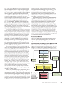
Figure 2. (a) ECA robotic setup, showing a sample, the robot tool-frame lifted away from the sample, and the structured-light camera facing the
sample, outside the robot’s workspace (b) ECA robotic scan on the sample (c) ECA probe view from below.
ME
|
ROBOTICECA
64
M AT E R I A L S E V A L U AT I O N • A P R I L 2 0 2 5

Preparation of Steel Samples with Corrosion Damage
A total of nine steel samples, each measuring 12 in. × 4 in.
(30.5 cm × 10.2 cm) were prepared for corrosion inspection
using the robotic ECA setup. The samples included three
distinct geometries: one flat, four concave, and four convex, as
shown in Figure 3. These shapes were achieved using a sheet
roller, with curvatures designed according to corrosion stan-
dards detailed in Table 1. After shaping, the samples underwent
a seven-day salt spray corrosion process in accordance with
ASTM B117-03 (ASTM 2003). To create a calibration area for the
ECA, the bottom inch (2.54 cm) of each sample was treated
with a corrosion inhibitor however, some corrosion leached
into this section. Residual rust was removed using a soaking
solution.
Comparison of Processed ECA Data with Microscope
Depth Profiling
Ground truth volumetric data of surface corrosion were
obtained using a high-resolution digital microscope for
comparison with the ECA data. To locate the defects,
2D cross-correlation was applied, in which the microscope
data was searched across the ECA data. The best matching
pattern was indicated by the maximum correlation value
between the two sets. The patterns from ECA voltages cor-
related well with the depths of the microscope data.
Challenges in Robotic ECA Inspection of Curved
Samples
Detecting fine surface or underpaint corrosion defects (e.g.,
50 µm deep) on curved metallic surfaces using robotic arms
is challenging due to strict liftoff, tilt, and thermal stability
requirements for the ECA probe. For example, ECT typically
necessitates maintaining a close and constant liftoff (e.g.,
1 mm) between the coil probe and the metallic surface. Small
liftoff ensures a noncontact testing method, maximizing the
induction of eddy currents and achieving a high signal-to-
noise ratio (SNR) for the measurements. Additionally, surface
corrosion detection often requires sensor coils to operate at
excitation frequencies in the MHz range. As a result, probe
misalignment and temperature fluctuations can introduce
errors during the scanning process, affecting both defect
detection and the accurate quantification of defect depth.
This section explores the challenges faced during robotic ECT
and presents typical experimental images obtained using the
proposed robotic NDE system with computer vision.
Effect of Inconsistent Probe Liftoff and Tilt on ECA
Measurements
Inconsistent liftoff typically introduces low spatial frequency
trends that overlap with defect indications, complicating image
processing and defect detection. Robotic manipulators can also
introduce inconsistent sensor tilt, affecting the distribution of
the excitation magnetic field from the coil sensor. For the rigid
and linear array probe, orientation errors affect each coil as a
body transformation, with coils at the edges of the array having
a different liftoff compared to the coils in its center. Improper
liftoff and/or tilt of the ECA probe can not only disrupt mea-
surements but also cause collisions with the test part, poten-
tially leading to immediate damage to the probe or long-term
degradation if dragged over rough surfaces.
B1 B2 B3 B4 C1 C2 C3 C4 A
Figure 3. Steel samples with corrosion damage: (a) flat sample A (b) concave samples B1–B4 (c) convex samples C1–C4.
TA B L E 1
Curvatures of test samples with corrosion damage
Sample A B1 B2 B3 B4 C1 C2 C3 C4
Curvature k (1/m) 0.000 0.304 0.397 0.527 0.842 0.304 0.451 0.528 0.842
A P R I L 2 0 2 5 • M AT E R I A L S E V A L U AT I O N 65