times, estimated the source location, and averaged the error in
distance over these 100 trials. This approach provides a solid
foundation for understanding the expected error range when
the agent has data from only three locations. The same meth-
odology was applied for scenarios with six, eight, and ten
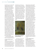
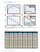
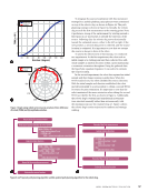
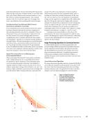
randomly chosen locations. Figure 6 illustrates the expected
error an agent might encounter when starting from differ-
ent grid points and selecting subsequent points at random.
The expected error is significantly higher in some cases,
primarily due to the agent’s potential vertical movement,
which increases the error. Although the expected error range
becomes narrower when the number of points is increased
to 10, the robot still expects a 120 mm to 140 mm error in
distance.
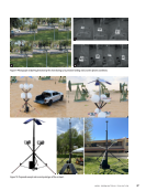
An alternative approach involves providing the agent
with additional information to enable more strategic
motion planning. This additional information is obtained
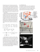
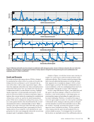
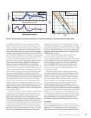
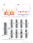
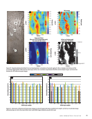
by rotating the microphone about the Z-axis. Figure 7 illus-
trates how the TDOA and amplitude change as the micro-
phones rotate. As expected, the TDOA reaches zero when
the robot is oriented directly toward the sound source
(leakage). While one may expect to receive the maximum
amplitude once the microphones are directed toward the
leakage source, our analysis shows that the maximum
amplitude slightly deviated from that direction, as depicted
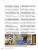
in Figure 7b. Consequently, starting from an initial position,
the robot can rotate about the Z-axis to accurately deter-
mine the direction of the sound source (leakage) when the
TDOA reaches zero. Once the direction is established, and
knowing that horizontal movement is more effective, the
robot can then move laterally to capture a second TDOA
reading and localize the sound location. This movement
strategy is tested using our robotic dog platform to replicate
more realistic scenarios.
ME
|
LEAKLOCALIZATION
1 0.25
0.2
0.15
0.1
0.05
2
3
4
5
6
7
8
–600
–800
–1000
–1200
–1400
X (mm)
–1600
–1800
–2000
–250 –200 –150 –100 –50 0 50 100
–600
–800
–1000
–1200
–1400
X (mm)
–1600
–1800
–2000
–250 –200 –150 –100 –50 0 50 100
8 7 6 5
X
4 3 2 1
1
0.2
0.3
0.4
0.5
0.6
0.1
2
3
4
5
6
7
8
8 7 6 5
X
4 3 2 1
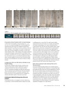
19.722
5
– 14.5775
14.5775
14.5–
77 5
– 14.5775
–
19.7225 19.7225
– 19.722
5
– 19.722
5 19.722 5
– 19.722
5
–
5
–
5
–
5
5
–19.722518.007
Leakage Leakage
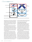
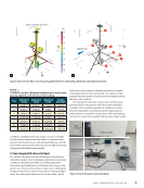
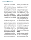
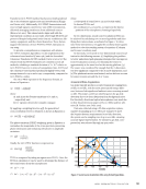
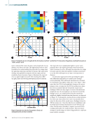
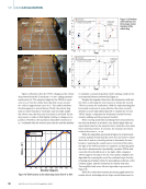
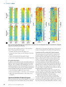
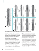
Figure 5. Distribution of error in the grid with the first location at (a) Point 1 and (b) Point 29. Intersection of hyperbolas constituted from points (c)
1 and 2, and (d) 1 and 9.
0.18
0.17
0.16
0.15
0.14
0.13
0.12
0.11
0.1
0.09 0 10 20 30 40 50 60 70
Location index
3 random points
6 random points
8 random points
10 random points
Figure 6. Expected error when the first position is fixed, and
subsequent points are chosen randomly.
56
M AT E R I A L S E V A L U AT I O N • A P R I L 2 0 2 5
Y
(mm)
Y
(mm)
Y Y
Expected
error
(m)
Error
(m)
Error
(m)

To integrate the source localization with this movement
strategy for a mobile platform, microphones were positioned
on top of the robotic dog, as shown in Figure 2b. The path
planning strategy is shown in Figure 8a. Initially, the robotic
dog records the first measurement at the starting point. Next,
it performs a sweep of the environment by rotating around a
fixed point in 15° increments to identify the direction of the
source. Following this, the robotic dog moves horizontally
toward the estimated source, either to the left or right. At the
new position, a second data point is collected, and the source
location is estimated. It is important to note that we assume
the source is always in front of the robot.
To assess the effectiveness of this strategy, we conducted
two experiments. In the first experiment, the robot took an
initial sample at a starting point and then collected two addi-
tional samples at random locations within a grid, maintaining
a consistent orientation throughout. Using the gathered data,
the hyperbolic equation (Equation 7) was solved to estimate
the source location.
In the second experiment, the robot first captured an initial
sample and then began rotating to gather data. When the
TDOA reached zero, the robot identified the source direction.
With the initial sample and direction established, the robot
moved horizontally to a new position to obtain a second TDOA
for source location estimation. It’s important to note that the
robot maintained the same orientation when taking the second
TDOA as it did for the first, as shown in Figure 9. Additionally,
the robotic dog’s rotational and translational movements
were executed manually rather than autonomously, with
the minimum step size for rotation being 15°. Figure 9 shows
the robotic dog’s motion trajectory for random and strategic
walking.
20
–2
–1
0
1
2
40 60 80 100 120 140 160
Direction θ (degrees)
180°
210° 330°
300° 240°
150°
120°
30°
60°
90°
0.8
0.6
0.4
0.2
1
270°
0°
Amplitude (v)
Leakage
TDOA trend
Leakage
Figure 7. Angle using robotic arm versus (a) variation of time difference
of arrival (TDOA) and (b) amplitude variation.
Record of the first measurement
Find sound source direction of arrival (DOA)
While (TDOA ≠ 0)
keep rotating about Z axis
if (TDOA =0)
DOA =current microphone orientation (θ)
If (0 DOA 90)
motion direction =right
If (90 DOA 180)
motion direction =left
Else
either direction is fine
If TDOA 0
motion direction =right
If T DOA 0
motion direction =left
Else
either direction is fine
Lateral motion direction
Lateral motion direction
Record of the second measurement
Record of the second measurement
Record of the first measurement
Estimate the source location
Estimate the source location
Figure 8. (a) Proposed path planning algorithm and (b) updated path planning algorithm for the robotic dog.
A P R I L 2 0 2 5 • M AT E R I A L S E V A L U AT I O N 57
TDOA
(s
×10–4)