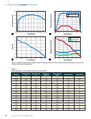
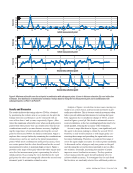
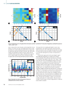
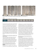
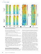
convex sample set C. In concave sample sets B2 and B3, the
right side of the scans shows saturation due to probe orienta-
tion errors, while set B4 displays desaturation across the entire
scan—an issue absent in the corresponding fast scan using the
same model. Fast scans experience similar tilting effects but
along the y-axis.
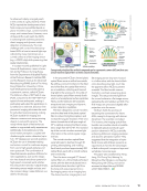
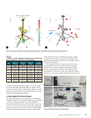
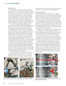
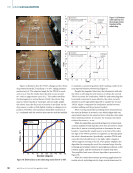
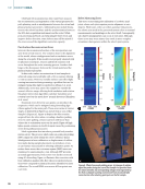
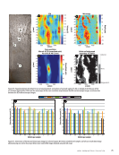
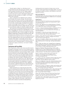
Comparison of ECA and Microscopic Data
The validation algorithm compares ECA scans of corroded
steel samples with corresponding microscopic images of cor-
rosion depth to assess the accuracy of the robotic NDE system.
Due to the time-intensive nature of microscopic imaging and
reconstruction, comparisons are performed only on randomly
selected regions of the test samples (D1–D4), as shown in
Figure 10a. The validation process follows these steps:
1. Data preprocessing. The microscopic data (Figure 10c)
is downsampled to match the pixel size of the ECA image
(Figure 10b), as the ECA scan covers a significantly larger area.
2. Alignment via cross-correlation. A cross-correlation
analysis is performed to align the datasets. The
algorithm searches within the ECA data, computes the
cross-correlation, and registers the location with the highest
match of image patterns, as illustrated in Figure 10d.
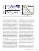
3. Defect identification. Once aligned, an intersection
operation is applied to identify defect regions. The ECA data
is thresholded, classifying values greater than zero as defects
(coded as “1”) and background areas as “0.” In contrast, the
microscopic data is thresholded such that values below zero
are marked as defects (“1”), while the background remains “0.”
4. Final classification. The binary masks from both datasets
are combined and averaged, as shown in Figure 10e. Defect
regions detected in both datasets are assigned a defect code
of “1” (white), background areas remain “0” (black), and
regions with no direct overlap receive an intermediate value
of “0.5” (gray). The percentage of intersection is then calcu-
lated, excluding the gray areas.
100
50
0
0
—0.1
—0.2
—0.3
—0.4
—0.5
0.1
0.2
0.3
0.4
0.5
x (mm)
A
1020 1040
—50
—100
100
50
0
0
—0.1
—0.2
—0.3
—0.4
—0.5
0.1
0.2
0.3
0.4
0.5
x (mm)
C1
1020 1040
—50
—100
100
50
0
0
—0.1
—0.2
—0.3
—0.4
—0.5
0.1
0.2
0.3
0.4
0.5
x (mm)
C2
—50
—100
100
50
0
0
—0.1
—0.2
—0.3
—0.4
—0.5
0.1
0.2
0.3
0.4
0.5
x (mm)
C3
1020 1040 1020 1040 1020 1040
—50
—100
100
50
0
0
—0.1
—0.2
—0.3
—0.4
—0.5
0.1
0.2
0.3
0.4
0.5
x (mm)
C4
—50
—100
100
50
0
0
—0.1
—0.2
—0.3
—0.4
—0.5
0.1
0.2
0.3
0.4
0.5
x (mm)
B1
1020 1040
—50
—100
100
50
0 0
—0.1
—0.2
—0.3
—0.4
—0.5
0.1
0.2
0.3
0.4
0.5
x (mm)
B2
—50
—100
100
50
0 0
—0.1
—0.2
—0.3
—0.4
—0.5
0.1
0.2
0.3
0.4
0.5
x (mm)
B3
1000 1020 1020 1040 1020 1040
—50
—100
100
50
0
0
—0.1
—0.2
—0.3
—0.4
—0.5
0.1
0.2
0.3
0.4
0.5
x (mm)
B4
—50
—100
Figure 9. Fast eddy current scans for steel samples: (a) flat sample A (b) concave samples B1–B4 (c) convex samples C1–C4.
ME
|
ROBOTICECA
70
M AT E R I A L S E V A L U AT I O N • A P R I L 2 0 2 5
V
(V)
Vo ltage
(V)
Vo ltage
(V)
Vo ltage
(V)
Vo ltage
(V)
Vo ltage
(V)
Vo ltage
(V)
Vo ltage
(V)
Vo ltage
(V)
y
(mm)
y
(mm)
y
(mm)
y
(mm)
y
(mm)
y
(mm)
y
(mm)
y
(mm)
y
(mm)

—40
—42
—44
—46
—48
—50
—52
—54
—56
—58
1030 1035 1040
—38
x (mm)
ECA
—40
—42
—44
—46
—48
—50
—52
—54
—56
—58
1030 1035 1040
—38
x (mm)
Microscope
0
—0.1
—0.2
—0.3
—0.4
—0.5
0.1
–5
—10
—15
—20
0
5
10
Defect int.
No int.
Background int.
15
20
0.2
0.3
0.4
0.5
—40
D4
D3
D2
D1
—42
—44
—46
—48
—50
—52
—54
—56
—58
1030 1035 1040
—38
x (mm)
Cross correlation
Max val: 0.539 (normalized units)
Pos [1035.8.-48.1] (mm)
—40
—42
—44
—46
—48
—50
—52
—54
—56
—58 1030 1035 1040
—38
x (mm)
Defect and background
interaction: 75.3895%
0
0.2
0.1
0.3
0.4
0.5
0.6
Figure 10. Experimental data for Defect D4 on corrosion Sample A: (a) locations of scanned regions D1–D4 on Sample A (b) ECA scan of D4
(c) corrosion depth profile of D4 from the microscope (d) the cross-correlation map between the ECA and microscopic images (e) intersection
between the ECA and microscopic images.
0
10
A B1 B2 B3 B4
Defects per sample
C1 C2 C3 C4
20
30
40
50
60
70
80
90
100
0
10
A B1 B2 B3 B4
Defects per sample
C1 C2 C3 C4
20
30
40
50
60
70
80
90
100
D1 D2 D3 D4 Not found
Figure 11. Intersection of the ECA and microscopic images in selected regions D1–D4 on corroded steel samples: (a) full scan results (ECA image
obtained using one coil in the array) (b) fast scan results (ECA image obtained using the full array).
A P R I L 2 0 2 5 • M AT E R I A L S E V A L U AT I O N 71
y
(mm)
y
(mm)
y
(mm)
y
(mm)
Intersection
percent
(%)
Intersection
percent
(%)
V
(V)
Depth
(μm)
Normalized
units