BCE is a loss function used in binary classification, where the
goal is to predict whether data instances belong to one of two
possible classes (e.g., underextrusion defect or no defect). In
contrast, CCE is used in multi-class classification scenarios (e.g.,
defect type), involving more than two classes. Both BCE and
CCE are fundamental in their respective domains, guiding the
model in adjusting its parameters to achieve optimal prediction
accuracy. To test the robustness of the proposed model, both
BCE and CCE were used to test single-defect and multi-defect
use cases. In the BCE loss function in Equation 2, the key vari-
ables include i the true label of each instance (0 or 1), and y,
the model’s predicted probability, indicating the likelihood that
the instance is in class 1. The function computes the average
loss over the total number of instances, using the natural
logarithm to intensify the penalty for confident but incorrect
predictions. In Equation 3, the CCE includes the true label
for each class of each instance, denoted as ij represented in
a one-hot encoded format, where it takes the value 1 for the
correct class and 0 for all other classes. The predicted proba-
bility that the th instance belongs to the th class is represented
by ˆij as estimated by the model. These probabilities should
sum to 1 across all classes for each instance. The CCE loss is
then averaged over N and summed across C, the total number
of classes, making it a comprehensive measure of the model’s
performance across all classes.
(2) BCE(y,ˆ) =− 1
N
∑ i=1[yi N *log(ˆ) + (1 − yi)*log(1 − ˆ )]
(3) CCE(y,ˆ) =− 1
N
∑
i=1
N ∑
j=1
C yijlog(ˆij)
Incorporating entropy regularization into BCE and CCE
introduces an additional term to the loss functions, aimed at
mitigating overconfidence in model predictions as a custom
loss function. In constructing the DEF, which integrates image
and waveform data, the complexity and the expansive number
of parameters pose a significant risk of overfitting. The inte-
gration of entropy regularization into the model’s learning
framework mitigated this risk by imposing constraints on the
model’s complexity. Given the intricate and nonlinear interde-
pendencies characterizing multimodal data, entropy regular-
ization played a vital role in preserving a degree of uncertainty
in the model’s predictions, thereby enhancing its robustness
to variations in input data. Moreover, challenges such as
sparse outputs or class imbalance, which can skew traditional
loss functions toward majority classes, necessitate the use of
entropy regularization. In addition, the inherent noise within
multimodal datasets, particularly those comprising disparate
data types such as images and waveforms, can detrimentally
affect model performance. Here, the inclusion of an entropy
term in the loss function can act as a buffer, promoting noise
robustness and discouraging overfitting to noisy data. These
factors collectively underscore the need for the custom loss
function with entropy regularization to foster a more general-
ized and reliable fusion model.
In its regularized form, with Equations 4 and 5, the custom
BCE ( c (y,ˆ) includes a regularization coefficient and the
average predicted probability ˆ to mitigate the model’s over-
confidence. It represents the average predicted probability
across all instances. The regularization term involves calcu-
lating the entropy of ˆ ( 1 (ˆ) which penalizes the model for
being too certain in its predictions. As the value increases,
the influence of entropy increases, leading to a more uniform
distribution and potentially underfitting the model. On the
other hand, as the value decreases, entropy exerts less influ-
ence, allowing the model to be more confident in its predic-
tions, which can lead to overfitting. For this study, was set to
0.3 so that the entropy regularization term contributes 30% to
the overall loss calculation. The value was chosen as it is sig-
nificant yet not an overwhelming portion, so that there was a
balance between following the training data (via primary loss
function) and maintaining uncertainty in the predictions (via
entropy).
(4) Bc(y, ˆ ) =− 1
N
∑ i=1[yi N *log(ˆ) + (1 − yi)*log(1 − ˆ )] − λ * E1 ( ˆ )
(5) E1(ˆ) = ˆ *log(ˆ) + (1 − ˆ )*log(1 − ˆ )
In the regularization variant of CCE, additional terms were
introduced to prevent overconfidence in predictions. Once
again, the regularization coefficient in Equation 6 deter-
mines the impact of regularization in the loss function. This
term uses ˆj the average predicted probability for each class
across all instances, to calculate the entropy of these proba-
bilities, as shown in Equation 7. The inclusion of this entropy
regularization term penalizes the model for predictions that
are too certain, encouraging a more balanced and generalized
approach in the model’s learning process, which is particularly
beneficial in complex multi-class classification tasks.
(6) CCE(y, )c =− 1
N
∑
i=1
N ∑
j=1
C yijlog( ij)− λ * E2 (ˆ)
(7) E2(ˆ) = ∑
j=1
C ˆ j log(ˆj)
2.3.2. DEF MODEL TRAINING
The overall approach is outlined in Figure 6a, starting with eval-
uating the single modality (images or time-series waveforms)
using state-of-the-art deep learning architectures. Each model
underwent hyperparameter tuning, including adjustments to
learning rate, batch size, number of epochs, activation func-
tions, dropout layers, regularization, and optimizer choices. The
optimal model was selected based on global and local metrics.
The architecture was then embedded in the DEF model frame-
work. The DEF model’s feature extraction layer was composed
of a deep learning architecture for images and time-series data,
respectively. To identify the most effective model, numerous
deep learning frameworks were tested, with hyperparameters
adjusted for each. These models were specifically chosen for
J U LY 2 0 2 6 • M AT E R I A L S E V A L U AT I O N 41
goal is to predict whether data instances belong to one of two
possible classes (e.g., underextrusion defect or no defect). In
contrast, CCE is used in multi-class classification scenarios (e.g.,
defect type), involving more than two classes. Both BCE and
CCE are fundamental in their respective domains, guiding the
model in adjusting its parameters to achieve optimal prediction
accuracy. To test the robustness of the proposed model, both
BCE and CCE were used to test single-defect and multi-defect
use cases. In the BCE loss function in Equation 2, the key vari-
ables include i the true label of each instance (0 or 1), and y,
the model’s predicted probability, indicating the likelihood that
the instance is in class 1. The function computes the average
loss over the total number of instances, using the natural
logarithm to intensify the penalty for confident but incorrect
predictions. In Equation 3, the CCE includes the true label
for each class of each instance, denoted as ij represented in
a one-hot encoded format, where it takes the value 1 for the
correct class and 0 for all other classes. The predicted proba-
bility that the th instance belongs to the th class is represented
by ˆij as estimated by the model. These probabilities should
sum to 1 across all classes for each instance. The CCE loss is
then averaged over N and summed across C, the total number
of classes, making it a comprehensive measure of the model’s
performance across all classes.
(2) BCE(y,ˆ) =− 1
N
∑ i=1[yi N *log(ˆ) + (1 − yi)*log(1 − ˆ )]
(3) CCE(y,ˆ) =− 1
N
∑
i=1
N ∑
j=1
C yijlog(ˆij)
Incorporating entropy regularization into BCE and CCE
introduces an additional term to the loss functions, aimed at
mitigating overconfidence in model predictions as a custom
loss function. In constructing the DEF, which integrates image
and waveform data, the complexity and the expansive number
of parameters pose a significant risk of overfitting. The inte-
gration of entropy regularization into the model’s learning
framework mitigated this risk by imposing constraints on the
model’s complexity. Given the intricate and nonlinear interde-
pendencies characterizing multimodal data, entropy regular-
ization played a vital role in preserving a degree of uncertainty
in the model’s predictions, thereby enhancing its robustness
to variations in input data. Moreover, challenges such as
sparse outputs or class imbalance, which can skew traditional
loss functions toward majority classes, necessitate the use of
entropy regularization. In addition, the inherent noise within
multimodal datasets, particularly those comprising disparate
data types such as images and waveforms, can detrimentally
affect model performance. Here, the inclusion of an entropy
term in the loss function can act as a buffer, promoting noise
robustness and discouraging overfitting to noisy data. These
factors collectively underscore the need for the custom loss
function with entropy regularization to foster a more general-
ized and reliable fusion model.
In its regularized form, with Equations 4 and 5, the custom
BCE ( c (y,ˆ) includes a regularization coefficient and the
average predicted probability ˆ to mitigate the model’s over-
confidence. It represents the average predicted probability
across all instances. The regularization term involves calcu-
lating the entropy of ˆ ( 1 (ˆ) which penalizes the model for
being too certain in its predictions. As the value increases,
the influence of entropy increases, leading to a more uniform
distribution and potentially underfitting the model. On the
other hand, as the value decreases, entropy exerts less influ-
ence, allowing the model to be more confident in its predic-
tions, which can lead to overfitting. For this study, was set to
0.3 so that the entropy regularization term contributes 30% to
the overall loss calculation. The value was chosen as it is sig-
nificant yet not an overwhelming portion, so that there was a
balance between following the training data (via primary loss
function) and maintaining uncertainty in the predictions (via
entropy).
(4) Bc(y, ˆ ) =− 1
N
∑ i=1[yi N *log(ˆ) + (1 − yi)*log(1 − ˆ )] − λ * E1 ( ˆ )
(5) E1(ˆ) = ˆ *log(ˆ) + (1 − ˆ )*log(1 − ˆ )
In the regularization variant of CCE, additional terms were
introduced to prevent overconfidence in predictions. Once
again, the regularization coefficient in Equation 6 deter-
mines the impact of regularization in the loss function. This
term uses ˆj the average predicted probability for each class
across all instances, to calculate the entropy of these proba-
bilities, as shown in Equation 7. The inclusion of this entropy
regularization term penalizes the model for predictions that
are too certain, encouraging a more balanced and generalized
approach in the model’s learning process, which is particularly
beneficial in complex multi-class classification tasks.
(6) CCE(y, )c =− 1
N
∑
i=1
N ∑
j=1
C yijlog( ij)− λ * E2 (ˆ)
(7) E2(ˆ) = ∑
j=1
C ˆ j log(ˆj)
2.3.2. DEF MODEL TRAINING
The overall approach is outlined in Figure 6a, starting with eval-
uating the single modality (images or time-series waveforms)
using state-of-the-art deep learning architectures. Each model
underwent hyperparameter tuning, including adjustments to
learning rate, batch size, number of epochs, activation func-
tions, dropout layers, regularization, and optimizer choices. The
optimal model was selected based on global and local metrics.
The architecture was then embedded in the DEF model frame-
work. The DEF model’s feature extraction layer was composed
of a deep learning architecture for images and time-series data,
respectively. To identify the most effective model, numerous
deep learning frameworks were tested, with hyperparameters
adjusted for each. These models were specifically chosen for
J U LY 2 0 2 6 • M AT E R I A L S E V A L U AT I O N 41