their proficiency in handling different aspects of time series and
image data, respectively.
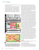
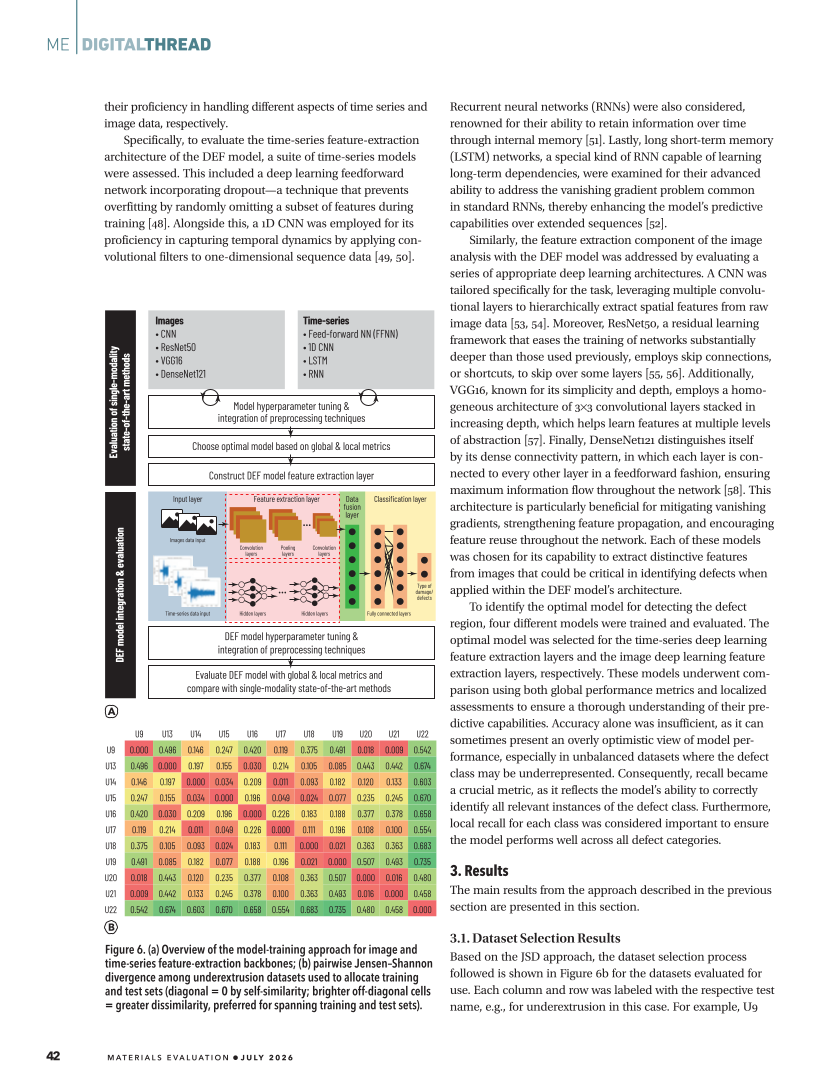
Specifically, to evaluate the time-series feature-extraction
architecture of the DEF model, a suite of time-series models
were assessed. This included a deep learning feedforward
network incorporating dropout—a technique that prevents
overfitting by randomly omitting a subset of features during
training [48]. Alongside this, a 1D CNN was employed for its
proficiency in capturing temporal dynamics by applying con-
volutional filters to one-dimensional sequence data [49, 50].
Recurrent neural networks (RNNs) were also considered,
renowned for their ability to retain information over time
through internal memory [51]. Lastly, long short-term memory
(LSTM) networks, a special kind of RNN capable of learning
long-term dependencies, were examined for their advanced
ability to address the vanishing gradient problem common
in standard RNNs, thereby enhancing the model’s predictive
capabilities over extended sequences [52].
Similarly, the feature extraction component of the image
analysis with the DEF model was addressed by evaluating a
series of appropriate deep learning architectures. A CNN was
tailored specifically for the task, leveraging multiple convolu-
tional layers to hierarchically extract spatial features from raw
image data [53, 54]. Moreover, ResNet50, a residual learning
framework that eases the training of networks substantially
deeper than those used previously, employs skip connections,
or shortcuts, to skip over some layers [55, 56]. Additionally,
VGG16, known for its simplicity and depth, employs a homo-
geneous architecture of 3×3 convolutional layers stacked in
increasing depth, which helps learn features at multiple levels
of abstraction [57]. Finally, DenseNet121 distinguishes itself
by its dense connectivity pattern, in which each layer is con-
nected to every other layer in a feedforward fashion, ensuring
maximum information flow throughout the network [58]. This
architecture is particularly beneficial for mitigating vanishing
gradients, strengthening feature propagation, and encouraging
feature reuse throughout the network. Each of these models
was chosen for its capability to extract distinctive features
from images that could be critical in identifying defects when
applied within the DEF model’s architecture.
To identify the optimal model for detecting the defect
region, four different models were trained and evaluated. The
optimal model was selected for the time-series deep learning
feature extraction layers and the image deep learning feature
extraction layers, respectively. These models underwent com-
parison using both global performance metrics and localized
assessments to ensure a thorough understanding of their pre-
dictive capabilities. Accuracy alone was insufficient, as it can
sometimes present an overly optimistic view of model per-
formance, especially in unbalanced datasets where the defect
class may be underrepresented. Consequently, recall became
a crucial metric, as it reflects the model’s ability to correctly
identify all relevant instances of the defect class. Furthermore,
local recall for each class was considered important to ensure
the model performs well across all defect categories.
3. Results
The main results from the approach described in the previous
section are presented in this section.
3.1. Dataset Selection Results
Based on the JSD approach, the dataset selection process
followed is shown in Figure 6b for the datasets evaluated for
use. Each column and row was labeled with the respective test
name, e.g., for underextrusion in this case. For example, U9
ME
|
DIGITALTHREAD
U9 U13 U14 U15 U16 U17 U18 U19 U20 U21 U22
U9 0.000 0.496 0.146 0.247 0.420 0.119 0.375 0.491 0.018 0.009 0.542
U13 0.496 0.000 0.197 0.155 0.030 0.214 0.105 0.085 0.443 0.442 0.674
U14 0.146 0.197 0.000 0.034 0.209 0.011 0.093 0.182 0.120 0.133 0.603
U15 0.247 0.155 0.034 0.000 0.196 0.049 0.024 0.077 0.235 0.245 0.670
U16 0.420 0.030 0.209 0.196 0.000 0.226 0.183 0.188 0.377 0.378 0.658
U17 0.119 0.214 0.011 0.049 0.226 0.000 0.111 0.196 0.108 0.100 0.554
U18 0.375 0.105 0.093 0.024 0.183 0.111 0.000 0.021 0.363 0.363 0.683
U19 0.491 0.085 0.182 0.077 0.188 0.196 0.021 0.000 0.507 0.493 0.735
U20 0.018 0.443 0.120 0.235 0.377 0.108 0.363 0.507 0.000 0.016 0.480
U21 0.009 0.442 0.133 0.245 0.378 0.100 0.363 0.493 0.016 0.000 0.458
U22 0.542 0.674 0.603 0.670 0.658 0.554 0.683 0.735 0.480 0.458 0.000
...
Input layer
Time-series data input
Images data input
Hidden layers Hidden layers Fully connected layers
Type of
damage/
defects
Feature extraction layer Data
fusion
layer
Classification layer
...
Convolution
layers
Convolution
layers
Pooling
layers
...
Images
• CNN
• ResNet50
• VGG16
• DenseNet121
Model hyperparameter tuning &
integration of preprocessing techniques
DEF model hyperparameter tuning &
integration of preprocessing techniques
Evaluate DEF model with global &local metrics and
compare with single-modality state-of-the-art methods
Choose optimal model based on global &local metrics
Construct DEF model feature extraction layer
Time-series
• Feed-forward NN (FFNN)
• 1D CNN
• LSTM
• RNN
Figure 6. (a) Overview of the model-training approach for image and
time-series feature-extraction backbones (b) pairwise Jensen–Shannon
divergence among underextrusion datasets used to allocate training
and test sets (diagonal =0 by self-similarity brighter off-diagonal cells
=greater dissimilarity, preferred for spanning training and test sets).
42
M AT E R I A L S E V A L U AT I O N • J U LY 2 0 2 6
Evaluation
of
single-modality
state-of-the-art
methods
DEF
model
integration
&
evaluation
image data, respectively.
Specifically, to evaluate the time-series feature-extraction
architecture of the DEF model, a suite of time-series models
were assessed. This included a deep learning feedforward
network incorporating dropout—a technique that prevents
overfitting by randomly omitting a subset of features during
training [48]. Alongside this, a 1D CNN was employed for its
proficiency in capturing temporal dynamics by applying con-
volutional filters to one-dimensional sequence data [49, 50].
Recurrent neural networks (RNNs) were also considered,
renowned for their ability to retain information over time
through internal memory [51]. Lastly, long short-term memory
(LSTM) networks, a special kind of RNN capable of learning
long-term dependencies, were examined for their advanced
ability to address the vanishing gradient problem common
in standard RNNs, thereby enhancing the model’s predictive
capabilities over extended sequences [52].
Similarly, the feature extraction component of the image
analysis with the DEF model was addressed by evaluating a
series of appropriate deep learning architectures. A CNN was
tailored specifically for the task, leveraging multiple convolu-
tional layers to hierarchically extract spatial features from raw
image data [53, 54]. Moreover, ResNet50, a residual learning
framework that eases the training of networks substantially
deeper than those used previously, employs skip connections,
or shortcuts, to skip over some layers [55, 56]. Additionally,
VGG16, known for its simplicity and depth, employs a homo-
geneous architecture of 3×3 convolutional layers stacked in
increasing depth, which helps learn features at multiple levels
of abstraction [57]. Finally, DenseNet121 distinguishes itself
by its dense connectivity pattern, in which each layer is con-
nected to every other layer in a feedforward fashion, ensuring
maximum information flow throughout the network [58]. This
architecture is particularly beneficial for mitigating vanishing
gradients, strengthening feature propagation, and encouraging
feature reuse throughout the network. Each of these models
was chosen for its capability to extract distinctive features
from images that could be critical in identifying defects when
applied within the DEF model’s architecture.
To identify the optimal model for detecting the defect
region, four different models were trained and evaluated. The
optimal model was selected for the time-series deep learning
feature extraction layers and the image deep learning feature
extraction layers, respectively. These models underwent com-
parison using both global performance metrics and localized
assessments to ensure a thorough understanding of their pre-
dictive capabilities. Accuracy alone was insufficient, as it can
sometimes present an overly optimistic view of model per-
formance, especially in unbalanced datasets where the defect
class may be underrepresented. Consequently, recall became
a crucial metric, as it reflects the model’s ability to correctly
identify all relevant instances of the defect class. Furthermore,
local recall for each class was considered important to ensure
the model performs well across all defect categories.
3. Results
The main results from the approach described in the previous
section are presented in this section.
3.1. Dataset Selection Results
Based on the JSD approach, the dataset selection process
followed is shown in Figure 6b for the datasets evaluated for
use. Each column and row was labeled with the respective test
name, e.g., for underextrusion in this case. For example, U9
ME
|
DIGITALTHREAD
U9 U13 U14 U15 U16 U17 U18 U19 U20 U21 U22
U9 0.000 0.496 0.146 0.247 0.420 0.119 0.375 0.491 0.018 0.009 0.542
U13 0.496 0.000 0.197 0.155 0.030 0.214 0.105 0.085 0.443 0.442 0.674
U14 0.146 0.197 0.000 0.034 0.209 0.011 0.093 0.182 0.120 0.133 0.603
U15 0.247 0.155 0.034 0.000 0.196 0.049 0.024 0.077 0.235 0.245 0.670
U16 0.420 0.030 0.209 0.196 0.000 0.226 0.183 0.188 0.377 0.378 0.658
U17 0.119 0.214 0.011 0.049 0.226 0.000 0.111 0.196 0.108 0.100 0.554
U18 0.375 0.105 0.093 0.024 0.183 0.111 0.000 0.021 0.363 0.363 0.683
U19 0.491 0.085 0.182 0.077 0.188 0.196 0.021 0.000 0.507 0.493 0.735
U20 0.018 0.443 0.120 0.235 0.377 0.108 0.363 0.507 0.000 0.016 0.480
U21 0.009 0.442 0.133 0.245 0.378 0.100 0.363 0.493 0.016 0.000 0.458
U22 0.542 0.674 0.603 0.670 0.658 0.554 0.683 0.735 0.480 0.458 0.000
...
Input layer
Time-series data input
Images data input
Hidden layers Hidden layers Fully connected layers
Type of
damage/
defects
Feature extraction layer Data
fusion
layer
Classification layer
...
Convolution
layers
Convolution
layers
Pooling
layers
...
Images
• CNN
• ResNet50
• VGG16
• DenseNet121
Model hyperparameter tuning &
integration of preprocessing techniques
DEF model hyperparameter tuning &
integration of preprocessing techniques
Evaluate DEF model with global &local metrics and
compare with single-modality state-of-the-art methods
Choose optimal model based on global &local metrics
Construct DEF model feature extraction layer
Time-series
• Feed-forward NN (FFNN)
• 1D CNN
• LSTM
• RNN
Figure 6. (a) Overview of the model-training approach for image and
time-series feature-extraction backbones (b) pairwise Jensen–Shannon
divergence among underextrusion datasets used to allocate training
and test sets (diagonal =0 by self-similarity brighter off-diagonal cells
=greater dissimilarity, preferred for spanning training and test sets).
42
M AT E R I A L S E V A L U AT I O N • J U LY 2 0 2 6
Evaluation
of
single-modality
state-of-the-art
methods
DEF
model
integration
&
evaluation