99.01%, 99.01%, and 96.16%, respectively. Macro F1, averaged
over defect and nondefect, is 99.50% for training and 99%,
99%, and 96% for U16, U17, and U18. For the multi-defect case
with three balanced classes, per-class recall alone does not
fix how errors split between the two incorrect labels, so we
report macro precision and macro F1 using a uniform split of
those errors across the other two classes. The corresponding
train and test values are 97.03% and 96.99%, and 96.83% and
96.62%, respectively.
In addition to evaluating the accuracy and recall for the
multi-defect case, the loss metric was also evaluated. The
loss performance heatmap in Figure 9b for the models indi-
cated that the DEF model was the optimal performer, with
the lowest loss values of 0.06 in both the training and test
datasets. This implied a robust model with a strong general-
ization capability, as it maintained consistent performance
from training to unseen data. In contrast, the CNN model with
processed images exhibited significantly higher loss values,
particularly with a loss of 3.45 on the training set and 2.37 on
the test set. This could indicate overfitting despite prepro-
cessing steps, as the model was penalized more heavily for
incorrect predictions, especially during training. The “Best: AE
DL” model showed moderate training and test losses of 0.79
and 0.59, respectively. Although not as low as the DEF model,
these values suggested a reasonable level of performance.
However, the relatively higher loss on the training set might
be due to underfitting, where the model may have been too
simple to capture the underlying patterns in the data. Finally,
the CNN model with raw images demonstrated a balanced
loss with 0.21 in training and a slightly higher 0.26 in testing.
This indicated a decent performance with some room for
improvement, especially in model generalization, to reduce the
increase in loss when evaluated on the test data.
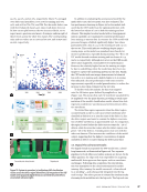
To further verify the analysis, the data was mapped
onto the AE feature space defined by amplitude vs. time
(Figure 10a). This means that each AE waveform was plotted by
its amplitude over the print duration, providing a visual repre-
sentation of the model’s classification results, where blue dots
represent nondefective waveforms and red dots denote defec-
tive waveforms.
The dotted line region represents when the defect region
occurred based on the G-code most of the waveforms were
classified as defective at or near the time of the defect. In fact,
the defect region was found to contain the highest concentra-
tion of defect waveforms, at approximately 25%. In comparison,
the region located before the defect area accounts for ~3% of
defects, while the area that comes after the defect region com-
prises ~9% of the defects. A similar pattern was seen with the
other test datasets. This increases the confidence of the model
output, suggesting that the highest concentration of signals
classified as defects occurred during the defect print time.
3.3. Digital Thread System Results
The digital thread incorporated the DEF model into a closed-
loop framework, as illustrated in Figure 10b. Two separate
pipelines for both offline and online analysis are shown. In the
offline pipeline, the edge node was responsible for acquiring
multimodal, heterogeneous data inputs, such as waveforms
and images. Following data acquisition, this raw informa-
tion was transmitted to the cloud environment for model
training. After training, the model was saved—often referred
to as “pickling”—and subsequently integrated into the fog
node’s script. The online process is initiated by simultaneously
streaming both modalities into the fog node. The fog node ran
Corrected region
Defect region
Defect region
Original print Corrected print during live test
1000 2000 3000 4000
65
60
55
50
45
40
35
Time (s)
No
Defectectf
dedefectecf
De
Edge node
...
Input layer
Time-series data input
Images data input
Hidden layers Hidden layers Fully connected layers
Type of
damage/ defects
Feature extraction layer Data fusion layer
Classification layer
...
Convulation layers Convulation layers Pooling layers
...
Cloud node
Model training
Fog node
Un-pickled data fusion model
Raw data
Raw data Save model
System feedback
Damage/defect
classification
Edge node
Multimodal NDE datasets
Multimodal NDE datasets
Data stream ...
Database, user dashboard,
model updating
Cloud node
Fog node
Pickled data fusion model
Figure 10. System in operation: (a) verification of AE classification
results across the defect region (dotted line) (b) integration of the DEF
model in the proposed digital thread (c) corrected live print (left) vs.
uncorrected reference (right).
J U LY 2 0 2 6 • M AT E R I A L S E V A L U AT I O N 47
Amplitude
(dB)
Offl.ligaine
Online
over defect and nondefect, is 99.50% for training and 99%,
99%, and 96% for U16, U17, and U18. For the multi-defect case
with three balanced classes, per-class recall alone does not
fix how errors split between the two incorrect labels, so we
report macro precision and macro F1 using a uniform split of
those errors across the other two classes. The corresponding
train and test values are 97.03% and 96.99%, and 96.83% and
96.62%, respectively.
In addition to evaluating the accuracy and recall for the
multi-defect case, the loss metric was also evaluated. The
loss performance heatmap in Figure 9b for the models indi-
cated that the DEF model was the optimal performer, with
the lowest loss values of 0.06 in both the training and test
datasets. This implied a robust model with a strong general-
ization capability, as it maintained consistent performance
from training to unseen data. In contrast, the CNN model with
processed images exhibited significantly higher loss values,
particularly with a loss of 3.45 on the training set and 2.37 on
the test set. This could indicate overfitting despite prepro-
cessing steps, as the model was penalized more heavily for
incorrect predictions, especially during training. The “Best: AE
DL” model showed moderate training and test losses of 0.79
and 0.59, respectively. Although not as low as the DEF model,
these values suggested a reasonable level of performance.
However, the relatively higher loss on the training set might
be due to underfitting, where the model may have been too
simple to capture the underlying patterns in the data. Finally,
the CNN model with raw images demonstrated a balanced
loss with 0.21 in training and a slightly higher 0.26 in testing.
This indicated a decent performance with some room for
improvement, especially in model generalization, to reduce the
increase in loss when evaluated on the test data.
To further verify the analysis, the data was mapped
onto the AE feature space defined by amplitude vs. time
(Figure 10a). This means that each AE waveform was plotted by
its amplitude over the print duration, providing a visual repre-
sentation of the model’s classification results, where blue dots
represent nondefective waveforms and red dots denote defec-
tive waveforms.
The dotted line region represents when the defect region
occurred based on the G-code most of the waveforms were
classified as defective at or near the time of the defect. In fact,
the defect region was found to contain the highest concentra-
tion of defect waveforms, at approximately 25%. In comparison,
the region located before the defect area accounts for ~3% of
defects, while the area that comes after the defect region com-
prises ~9% of the defects. A similar pattern was seen with the
other test datasets. This increases the confidence of the model
output, suggesting that the highest concentration of signals
classified as defects occurred during the defect print time.
3.3. Digital Thread System Results
The digital thread incorporated the DEF model into a closed-
loop framework, as illustrated in Figure 10b. Two separate
pipelines for both offline and online analysis are shown. In the
offline pipeline, the edge node was responsible for acquiring
multimodal, heterogeneous data inputs, such as waveforms
and images. Following data acquisition, this raw informa-
tion was transmitted to the cloud environment for model
training. After training, the model was saved—often referred
to as “pickling”—and subsequently integrated into the fog
node’s script. The online process is initiated by simultaneously
streaming both modalities into the fog node. The fog node ran
Corrected region
Defect region
Defect region
Original print Corrected print during live test
1000 2000 3000 4000
65
60
55
50
45
40
35
Time (s)
No
Defectectf
dedefectecf
De
Edge node
...
Input layer
Time-series data input
Images data input
Hidden layers Hidden layers Fully connected layers
Type of
damage/ defects
Feature extraction layer Data fusion layer
Classification layer
...
Convulation layers Convulation layers Pooling layers
...
Cloud node
Model training
Fog node
Un-pickled data fusion model
Raw data
Raw data Save model
System feedback
Damage/defect
classification
Edge node
Multimodal NDE datasets
Multimodal NDE datasets
Data stream ...
Database, user dashboard,
model updating
Cloud node
Fog node
Pickled data fusion model
Figure 10. System in operation: (a) verification of AE classification
results across the defect region (dotted line) (b) integration of the DEF
model in the proposed digital thread (c) corrected live print (left) vs.
uncorrected reference (right).
J U LY 2 0 2 6 • M AT E R I A L S E V A L U AT I O N 47
Amplitude
(dB)
Offl.ligaine
Online