indicates the underextrusion test 9. Based on the dataset com-
parison, a value of 0 denotes perfect self-similarity. In general,
a lower JSD value indicates higher similarity, while a higher
value suggests greater dissimilarity between datasets. Based on
the results of the JSD analysis, selecting U15, U19, and U13 for
the training set and U16, U17, and U18 for the test set creates
a strategic balance that helps the model learn effectively by
leveraging both similarities and diversities within the data. A
more diverse training dataset, such as the combination of U15,
U19, and U13, generally leads to improved model performance
by presenting a wider array of examples for learning and better
generalization. On the other hand, U16, U17, and U18 show
greater dissimilarity from the training datasets, making them
appropriate for testing. This ensures that the model is tested
against patterns that are significantly different from those
encountered during training, providing a stringent assessment
of its ability to generalize to new data. Success in accurately
predicting these dissimilar patterns would indicate that the
model has not only learned the underlying structures in the
training data but can also apply this knowledge to previously
unseen instances. By keeping the testing datasets separate and
diverse, the model’s performance evaluation remains objec-
tive and provides a credible measure of its robustness. The
colormap of the divergence matrix has been updated for clarity
per reviewer feedback so that highly similar (low-JSD) cells are
visually distinct from highly dissimilar cells.
To maintain consistency and balance within the dataset,
the minimum common frame count across these sets was
identified to be 50. Consequently, this established the baseline
for both the defective and nondefective layers, ensuring an
equitable distribution of data for model training and testing.
Hence, the specific pairs of waveform and corresponding
images used are listed in Table 4. For example, for U13, there
were 50 images and 50 corresponding waveforms for the
no-defect class. Conversely, there were 50 images and corre-
sponding waveforms for the defect class.
To extend this work, the multi-defect use case was devel-
oped as well. For the multi-defect case, warping datasets were
added to the underextrusion datasets for training and testing,
as shown in Table 5.
3.2. DEF Model Results
Based on the trained models in Figure 6a, the optimal model
for images was a convolutional neural network (CNN), while
the optimal model for time-series datasets was a feedforward
neural network (FFNN). The optimal models were selected
through a series of hyperparameter tuning, ensuring consis-
tent results across the training and test datasets, with a focus
on both global and local metrics, such as accuracy and recall.
The architecture shown in Figure 5b delineates the multi-input
neural network tailored for processing image and time-series
waveform data. The image data passes through a custom
CNN comprising two convolutional layers, each followed by a
max pooling layer to downsample the image while preserving
essential features. The resulting feature maps are then flattened
into a single vector. Concurrently, the time-series waveform
data is processed by a feedforward neural network, beginning
with an input layer and followed by a dense layer to capture
temporal dependencies. The outputs of both the CNN and
the feedforward network are concatenated to form a unified
feature vector, which is then fed into a final dense layer to
produce the system’s output.
The training hyperparameters for the DEF utilized the
Adam optimizer. The learning rate was set to a conservative
value of 0.00001, with the first moment decay rate 1 at 0.9
and the second moment decay rate 2 at 0.99, a configura-
tion that helps smooth the trajectory toward the minimum.
The network was trained for 5 epochs with a batch size of 2
to refine gradient updates and manage memory efficiently.
The training data was shuffled, ensuring that each batch pre-
sented a diverse set of samples to the model, which is critical
for preventing the model from learning spurious patterns.
TA B L E 4
Dataset selection for the single-defect case
Training data
Test no. No defect Defect: Underextrusion
U13 50 50
U15 50 50
U19 50 50
Testing data
Test no. No defect Defect: Underextrusion
U16 50 50
U17 50 50
U18 50 50
TA B L E 5
Dataset selection for the multi-defect case
Training data
Test no. No defect Defect: Underextrusion Defect: Warping
W1 50 x 50
W2 50 x 50
U13 50 50 x
U15 50 50 x
Testing data
Test no. No defect Defect: Underextrusion Defect: Warping
W3 50 x 50
U16 50 50 x
J U LY 2 0 2 6 • M AT E R I A L S E V A L U AT I O N 43
parison, a value of 0 denotes perfect self-similarity. In general,
a lower JSD value indicates higher similarity, while a higher
value suggests greater dissimilarity between datasets. Based on
the results of the JSD analysis, selecting U15, U19, and U13 for
the training set and U16, U17, and U18 for the test set creates
a strategic balance that helps the model learn effectively by
leveraging both similarities and diversities within the data. A
more diverse training dataset, such as the combination of U15,
U19, and U13, generally leads to improved model performance
by presenting a wider array of examples for learning and better
generalization. On the other hand, U16, U17, and U18 show
greater dissimilarity from the training datasets, making them
appropriate for testing. This ensures that the model is tested
against patterns that are significantly different from those
encountered during training, providing a stringent assessment
of its ability to generalize to new data. Success in accurately
predicting these dissimilar patterns would indicate that the
model has not only learned the underlying structures in the
training data but can also apply this knowledge to previously
unseen instances. By keeping the testing datasets separate and
diverse, the model’s performance evaluation remains objec-
tive and provides a credible measure of its robustness. The
colormap of the divergence matrix has been updated for clarity
per reviewer feedback so that highly similar (low-JSD) cells are
visually distinct from highly dissimilar cells.
To maintain consistency and balance within the dataset,
the minimum common frame count across these sets was
identified to be 50. Consequently, this established the baseline
for both the defective and nondefective layers, ensuring an
equitable distribution of data for model training and testing.
Hence, the specific pairs of waveform and corresponding
images used are listed in Table 4. For example, for U13, there
were 50 images and 50 corresponding waveforms for the
no-defect class. Conversely, there were 50 images and corre-
sponding waveforms for the defect class.
To extend this work, the multi-defect use case was devel-
oped as well. For the multi-defect case, warping datasets were
added to the underextrusion datasets for training and testing,
as shown in Table 5.
3.2. DEF Model Results
Based on the trained models in Figure 6a, the optimal model
for images was a convolutional neural network (CNN), while
the optimal model for time-series datasets was a feedforward
neural network (FFNN). The optimal models were selected
through a series of hyperparameter tuning, ensuring consis-
tent results across the training and test datasets, with a focus
on both global and local metrics, such as accuracy and recall.
The architecture shown in Figure 5b delineates the multi-input
neural network tailored for processing image and time-series
waveform data. The image data passes through a custom
CNN comprising two convolutional layers, each followed by a
max pooling layer to downsample the image while preserving
essential features. The resulting feature maps are then flattened
into a single vector. Concurrently, the time-series waveform
data is processed by a feedforward neural network, beginning
with an input layer and followed by a dense layer to capture
temporal dependencies. The outputs of both the CNN and
the feedforward network are concatenated to form a unified
feature vector, which is then fed into a final dense layer to
produce the system’s output.
The training hyperparameters for the DEF utilized the
Adam optimizer. The learning rate was set to a conservative
value of 0.00001, with the first moment decay rate 1 at 0.9
and the second moment decay rate 2 at 0.99, a configura-
tion that helps smooth the trajectory toward the minimum.
The network was trained for 5 epochs with a batch size of 2
to refine gradient updates and manage memory efficiently.
The training data was shuffled, ensuring that each batch pre-
sented a diverse set of samples to the model, which is critical
for preventing the model from learning spurious patterns.
TA B L E 4
Dataset selection for the single-defect case
Training data
Test no. No defect Defect: Underextrusion
U13 50 50
U15 50 50
U19 50 50
Testing data
Test no. No defect Defect: Underextrusion
U16 50 50
U17 50 50
U18 50 50
TA B L E 5
Dataset selection for the multi-defect case
Training data
Test no. No defect Defect: Underextrusion Defect: Warping
W1 50 x 50
W2 50 x 50
U13 50 50 x
U15 50 50 x
Testing data
Test no. No defect Defect: Underextrusion Defect: Warping
W3 50 x 50
U16 50 50 x
J U LY 2 0 2 6 • M AT E R I A L S E V A L U AT I O N 43