increase in amplitude. The burst signified an intense release
of energy, followed by a swift return to baseline—a pattern
that was distinct from the characteristics of a nondefective
waveform. The representative waveform from the nondefect
region was found to be more continuous.
To verify the robustness of the deep learning models,
a series of preprocessing steps was applied to enhance the
quality and suitability of the images. Specifically, the model
evaluations presented in the results section include metrics
computed from both preprocessed and raw images for com-
parison. There were two major preprocessing steps. The first
step involved image enhancement to address variations in
lighting conditions that could affect the model’s performance.
This initial enhancement standardized the images, making
them more consistent for subsequent processing. Following
image enhancement, a color thresholding step was applied to
the images. This process was instrumental in isolating specific
color ranges of interest, such as light green. By defining the
lower and upper bounds in terms of hue, saturation, and value
(HSV) specific to the desired color range, the images were trans-
formed into a format that retained only the targeted colors.
For image enhancement, the histogram equalization
method was used. Initially, the images were converted from
the BGR (blue, green, red) color space to YUV, separating the
luminance (Y) and chrominance (U, V) components. This sep-
aration allowed for independent processing of brightness and
color information. Histogram equalization was then applied
exclusively to the luminance channel (Y) to enhance contrast
and brightness without altering the color relationships within
the image. This approach is a standard practice in image pro-
cessing when the primary goal is to improve contrast while
preserving color fidelity. The equalized Y channel in the YUV
color space was subsequently transformed back to the BGR
color space, ensuring the images retained their original format.
To further enhance image quality, a series of histogram-based
steps was performed. These steps included calculating the his-
togram of the input image, computing the cumulative distribu-
tion function (CDF) to understand pixel intensity distribution,
ME
|
DIGITALTHREAD
Time (s)
65
60
55
50
45
40
0 1000 2000 3000 4000
Selected defect S ssignallig
Time (s)
65
60
55
50
45
40
0 1000 2000 3000 4000
Selected pristine signaligs S pristine
Time (uni00B5s)
0.03
0.02
0.01
0.00
–0.01
–0.02
–0.03
0 200 400 600 800 1000
Time (uni00B5s)
0.0100
0.0075
0.0050
0.0025
0.0000
–0.0025
–0.0050
–0.0075
0 200 400 600 800 1000
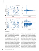
Figure 3. Representative AE waveforms: (a) defect region (burst-like, with sharp amplitude rise and rapid decay) (b) nondefect region (more
continuous behavior).
38
M AT E R I A L S E V A L U AT I O N • J U LY 2 0 2 6
Amplitude
(dB)
Amplitude
(dB)
Voltage
(V)
Voltage
(V)
of energy, followed by a swift return to baseline—a pattern
that was distinct from the characteristics of a nondefective
waveform. The representative waveform from the nondefect
region was found to be more continuous.
To verify the robustness of the deep learning models,
a series of preprocessing steps was applied to enhance the
quality and suitability of the images. Specifically, the model
evaluations presented in the results section include metrics
computed from both preprocessed and raw images for com-
parison. There were two major preprocessing steps. The first
step involved image enhancement to address variations in
lighting conditions that could affect the model’s performance.
This initial enhancement standardized the images, making
them more consistent for subsequent processing. Following
image enhancement, a color thresholding step was applied to
the images. This process was instrumental in isolating specific
color ranges of interest, such as light green. By defining the
lower and upper bounds in terms of hue, saturation, and value
(HSV) specific to the desired color range, the images were trans-
formed into a format that retained only the targeted colors.
For image enhancement, the histogram equalization
method was used. Initially, the images were converted from
the BGR (blue, green, red) color space to YUV, separating the
luminance (Y) and chrominance (U, V) components. This sep-
aration allowed for independent processing of brightness and
color information. Histogram equalization was then applied
exclusively to the luminance channel (Y) to enhance contrast
and brightness without altering the color relationships within
the image. This approach is a standard practice in image pro-
cessing when the primary goal is to improve contrast while
preserving color fidelity. The equalized Y channel in the YUV
color space was subsequently transformed back to the BGR
color space, ensuring the images retained their original format.
To further enhance image quality, a series of histogram-based
steps was performed. These steps included calculating the his-
togram of the input image, computing the cumulative distribu-
tion function (CDF) to understand pixel intensity distribution,
ME
|
DIGITALTHREAD
Time (s)
65
60
55
50
45
40
0 1000 2000 3000 4000
Selected defect S ssignallig
Time (s)
65
60
55
50
45
40
0 1000 2000 3000 4000
Selected pristine signaligs S pristine
Time (uni00B5s)
0.03
0.02
0.01
0.00
–0.01
–0.02
–0.03
0 200 400 600 800 1000
Time (uni00B5s)
0.0100
0.0075
0.0050
0.0025
0.0000
–0.0025
–0.0050
–0.0075
0 200 400 600 800 1000
Figure 3. Representative AE waveforms: (a) defect region (burst-like, with sharp amplitude rise and rapid decay) (b) nondefect region (more
continuous behavior).
38
M AT E R I A L S E V A L U AT I O N • J U LY 2 0 2 6
Amplitude
(dB)
Amplitude
(dB)
Voltage
(V)
Voltage
(V)