Transform (GCC-PHAT) method has become widely preferred
due to its robustness against noise and reverberation (Knapp
and Carter 1976). Additionally, GCC-PHAT demonstrates resil-
ience in high signal-to-interference ratio (SIR) environments,
effectively managing interference from additional sources
(Kwon et al. 2010). This characteristic aligns well with the
experimental conditions in our study, where high SIR levels are
preserved despite background noise from air conditioners, lab-
oratory equipment, and the robots themselves. These factors
support the selection of GCC-PHAT for TDOA estimation in
our setup.
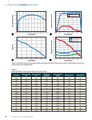
To provide a comprehensive comparison with alterna-
tive TDOA estimation algorithms, we also implemented the
coherence-based method (Carter 1987) and the Smoothed
Coherence Transform (SCOT) method (Carter et al. 1973). The
results reveal that TDOA estimates are consistent across all
methods, exhibiting a standard deviation of ​ × ​ 10​​−6​​ relative to
GCC-PHAT. However, in terms of computation time, SCOT and
the coherence-based method performed slightly better, with
average times of 0.050 s and 0.0519 s, respectively, compared to
GCC-PHAT’s 0.0685 s.
The GCC-PHAT operates in the frequency domain, as
shown in Equation 2: ​ ​
(2)​ ​ CCF​[f]​ =A1​[f]​A2​[f]​​​*​​
where ​
A1​ and ​ 2​ are the Fourier transforms of ​​ ​ 1​​​ and ​​ ​ 2​​​ ,
respectively, and
the {.}*operator denotes the complex conjugate.
By applying a weighting function ​​ ​ [​​f]​​​​ ​ the generalized
cross-correlation (GCC) is obtained, as shown in Equation 3: ​ ​
(3)​ GCCF​[f]​ =ψ​[f]​​A1​[f]​A2​[​​f​]​​​​*​​
The phase transform (PHAT) weighting, given in Equation 4,
normalizes the magnitude of the cross-spectrum, preserving
phase information and enhancing robustness to amplitude
variations: ​ ​
(4)​ ψ​[f]​ =​ 1 _​
|A1​[f]​A2​[​​f​]​​​​*​|​​​ ​
Finally, the GCC-PHAT function is expressed as: ​ ​
(5)​ PHA​TF​​​[f]​ ​ =​ ​ A1​[f]​A2​[​​f​]​​​​*​ _​
|A1​[f]​A2​[​​f​]​​​​*​|​​​​
TDOA is computed by taking an argmax over ​ HA​TF​​​ ​ Once the
TDOA is calculated, it can be used to determine the distance of
the sound source from the microphones: ​ ​
(6)​ ∆d =c *∆ t​ ​ ​
(7)​ ∆d =​ √
__________________​ ​ ​
(​​x​2​​ − x​)​​​​2​ − ​ ​ ​ (​​y2​​ ​ − y​)​​​​2​​ − ​ √
__________________​​​
(​​x1​​ ​ − x​)​​​​2​ − ​ ​ ​ (​​y1​​ ​ − y​)​​​​2​​​
where​
c​ is the speed of sound (set to 343 m/s for this study),
∆t denotes TDOA, and
the coordinates (​​ ​ 1​​​ ​​ ​ 1​​​ and (​​ ​ 2​​​ ​​ ​ 2​​​ represent the known
positions of the microphones, forming a hyperbola.
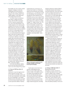
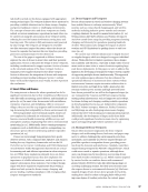
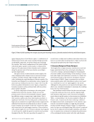
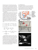
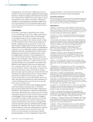
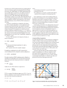
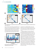
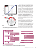
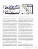
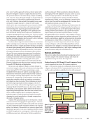
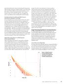
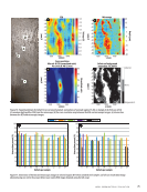
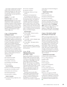
In two dimensions, sound source localization (SSL) can
be achieved by calculating two or more hyperbolas and iden-
tifying their intersections, as indicated in Figure 1. To deter-
mine these intersections, we apply the nonlinear least-squares
method to solve the resulting system of equations (Coleman
and Li 1996 Levenberg 1944).
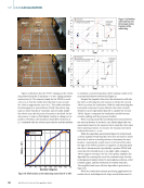
In this study, we focused on two-dimensional source local-
ization for the following reasons: (1) Simplifying the problem
to better understand path planning strategies that can improve
source localization accuracy, (2) Assuming the source is
approximately at the same level as the moving platform, (3)
The source was considered far enough that the Z-dimension
was less significant compared to the X and Y dimensions, and
(4) The platform’s motion was limited, and we did not account
for sensor rotation around the X or Y axes.
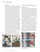
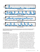
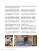
Acoustical Data Acquisition
Gas leaks typically produce acoustic frequencies ranging from
10 kHz to 100 kHz, with the most pronounced energy differ-
ence between leak signals and ambient noise occurring around
40 kHz. This makes 40 kHz an ideal frequency for gas leak
detection due to its clear distinction from background noise.
For this study, directional optical microphones were used due
to their broad detection range (10 Hz to 1 MHz) and low self-
noise (B. Fischer 2016 Delic 2019).
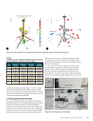
Data was collected using a NI data acquisition system,
capable of sampling up to 20 MS/s per channel. To meet
the Nyquist theorem requirements for 40 kHz detection,
the system used a sampling rate of up to 400 kHz, ensuring
accurate signal representation. To simulate a gas leak, com-
pressed air was released through an open valve.
–600
–250 –200 –150 –100 –50 0 50 100
–800
–1000
–1200
–1400
–1600
–1800
X (mm)
–2000
10.29
1 0.2
9 –1 0
.29
–10
.2
9
– 10.2
9
–1 0.29
10.2 9
10.2 9
–19.7225
–19
.7 225
–1 9. 7225
–19.7
22 5
1 9.722
5
Estimated location
Sound source
Error
M1 M1 M2
M2
Figure 1. Sound source localization (SSL) using formed hyperbolas.
A P R I L 2 0 2 5 • M AT E R I A L S E V A L U AT I O N 53
Y
(mm)

Robotic System
To explore the impact of dynamic motion on gas leakage
source localization, two robotic systems equipped with micro-
phones were used: a fixed-based robotic arm and a quadruped
robot (robotic dog). The robotic arm, a collaborative robotic
arm developed by Universal Robots and known for its pre-
cision and repeatability (±0.03 mm), was used to study the
effects of translational and rotational microphone motions
while the sound source remained fixed. Its high accuracy
supports the development of localization algorithms by min-
imizing estimation errors. However, its fixed-base design and
850 mm reach limit its applicability in industrial settings.
In contrast, the robotic dog, a quadrupedal robotic
platform, is more suitable for deployment in industrial settings.
This robotic dog is equipped with a 16-channel lidar and
a depth camera. It can map the environment, detect pipe-
lines with potential gas leakage, and generate depth maps
for precise localization. Its ability to navigate varying terrains
enables broader coverage for gas leak detection. It can also be
enhanced with biomimetic pinnae-like structures, mimick-
ing feline ear movements (yaw, pitch, roll, and independent
motion) to improve sound localization by capturing multiple
acoustic samples in complex settings. This enhancement
presents an intriguing direction for future work, as the findings
of Ruhland et al. (2015) suggest that the coordinated movements
of a cat’s head and pinna enable the collection of multiple
acoustic samples to improve sound localization accuracy. This
also introduces the possibility of fully emulating animal head
and ear movements for enhanced sound source localization.
Although we attempted to incorporate feline pinnae and head
movements into our system, the inconsistency and unreliability
of the data, compared to findings from Young et al. (1996), pre-
vented us from achieving the desired results.
For the initial study, the microphones were mounted
on a custom plate attached to the robotic arm, as shown in
Figure 2a. Positioned 90 mm apart on a circular disc, they
mimic the locations of feline pinnae. A similar mounting
bracket was created to hold and position the two microphones
on the back of the robotic dog, as depicted in Figure 2b.
Experimental Setup
Biological creatures like cats and dogs rotate their heads or
move their bodies to localize sound sources and enhance the
TDOA of sound waves at their ears. These movements improve
auditory cues that the brain uses to determine the direction
and distance of a sound. When a sound originates from one
side, it reaches the nearer ear slightly earlier than the farther
ear. This small difference in time, known as the interaural time
difference (ITD), helps the brain determine the direction of the
sound source. By moving their heads or bodies, these creatures
change the relative position of their ears to the sound source,
creating different TDOA patterns that provide additional spatial
cues for more accurate localization.
To replicate these complex motions in a simplified manner,
they are divided into linear and rotational components. For
linear movements, microphones were mounted on the robotic
arm’s end-effector. The arm followed a linear path using a
linear path planner (MoveL), traversing an 8 ​ ×​ 8 grid with
50 mm increments along the X and Y axes. This systematic
movement covered the designated area for sound localization
experiments, with the sound source positioned 1.79 m from the
robotic arm’s base along the Y-axis, as shown in Figure 3a.
Rotational movements were also replicated in a separate
experiment to mimic the head-turning behavior of biological
creatures during sound localization. Microphones mounted
on the robotic arm’s end-effector were rotated along the Z-axis
from 10° to 170° in 5° increments, as shown in Figure 3b. This
systematic variation in microphone orientation was designed
to evaluate how angular positioning affects the TDOA and
enhances the accuracy of determining the direction of arrival
(DOA) of sound.
ME
|
LEAKLOCALIZATION
Leakage
Distance =1790 mm
θ =10°
θ =170°
Δθ =5°
Δx =50 mm
Δy =50 mm Point 64
Point 1
y
x
y
x
Figure 3. Movement of robotic arm: (a) linear along the X and Y axes
(b) rotational around the Z-axis.
3D printed handle
Lidar
Depth camera
z
x
y
90 mm
3D printed handle
90 mm
z x
y
Figure 2. Microphone attachments to (a) the robotic arm and (b) the robotic dog.
54
M AT E R I A L S E V A L U AT I O N • A P R I L 2 0 2 5