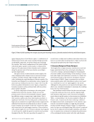
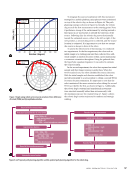
particularly affecting the Denavit–Hartenberg (DH) parameters
rather than the Cartesian coordinate system, as seen with other
error types. These calibration inaccuracies manifest as “wave-
like” patterns, introducing approximately 1 mm of spatial
variance in the ECA scans (see Figure 6a). To mitigate this
issue, a specialized post-processing method was developed.
Synchronization Error Between Eddy Current
Instrument and Robot’s Controller
Errors arising from poor synchronization between the robot’s
real-time orientation data and the real-time acquisition of
the scanning instrument must also be considered. These syn-
chronization issues cause smearing due to lag between the
two data streams. The system managing both data flows—
comprising the robot’s controller and the ECA data acquisi-
tion instrument—operates as two separate systems, leading to
inevitable delays. Although timestamps are recorded alongside
each data stream, a nonconstant delay persists between the
two. On average, this delay was found to be approximately
50 ms. To minimize the effects of this delay, slower scan speeds
of 25 mm/s were employed, reducing smearing to under 1 mm,
which was adequate to detect most corrosion flaws.
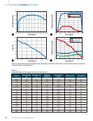
Signal Fluctuation Due to Coil Heating and
Environmental Effects
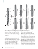
When performing NDE using ECT array probes in absolute
mode, voltage fluctuations are occasionally observed that
are unrelated to probe orientation. These fluctuations may
occur even when the probe is stationary. Such behavior is
typically attributed to high excitation currents in the coils or
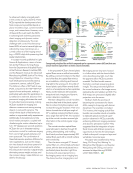
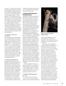
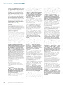
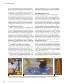
ambient temperature changes (García-Martín et al. 2011). For
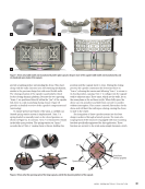
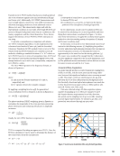
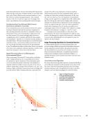
instance, Figure 5 illustrates a pronounced case of voltage drift
in an ECA probe while it remains stationary 1 mm above the
sample. This drift occurs during the coil warm-up phase
after powering on the ECA data acquisition system, prior to
reaching its steady-state operating temperature. In this case,
the coils were driven at twice the maximum recommended
voltage, and the signals were amplified by 60 dB. Additionally,
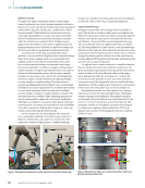
the robot, ECA probe, and steel test sample with corrosion
damage were situated near a high-power air duct emitting hot
air into the adjacent lab space. Once the coils reached their
steady-state temperature, the ECA probe was nulled on an
undamaged region of the test sample. After calibration, voltage
variations were reduced to a range of –0.015 V to 0.015 V.
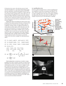
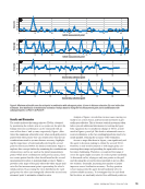
To mitigate environmental effects on the robotic ECA
measurements, the system was programmed to null the array
probe in the damage-free region at fixed intervals. Additionally,
a second-order detrending process was applied to each coil
signal in the time domain.
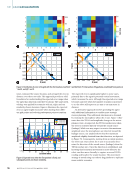
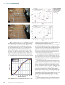
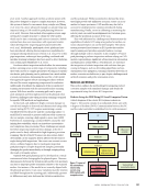
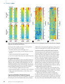
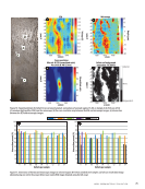
Image Processing Algorithms for Corrosion Detection
To address liftoff variations and environmental effects, the
post-processing workflow incorporates a specialized array sub-
traction algorithm and detrending. This approach leverages
the shared liftoff errors across the coils to isolate and correct
these inconsistencies effectively. A simplified representation
of the post-processing procedure is provided in Figure 6. A
detailed description can be found in the authors’ previous work
(Hamilton 2024).
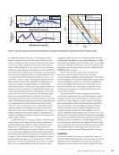
Array Subtraction Algorithm
The array subtraction algorithm removes common liftoff effects
across all probe channels by subtracting the mean value of the
line scans, effectively eliminating identical noise and voltage
variations between coils. It is applied to ECA data in the time
domain to prevent spatial misalignment caused by delays
0 1
—40
—35
—300
—25
—20
—15
—10
—5
0
5
2 3 4 5 6 7
1
2
3
4
5
6
7
8
9
10
11
12
13
14
15
16
17
18
19
20
21
22
23
24
25
26
27
28
29
30
31
32
Time
Coils
0
—
—
0
5
0
—
((min)n
Figure 5. Voltage fluctuations
in the coils (absolute mode)
caused by array probe heating
during warm-up and hot air
circulation around the probe.
A P R I L 2 0 2 5 • M AT E R I A L S E V A L U AT I O N 67
V
(V)
o
geoltage
rather than the Cartesian coordinate system, as seen with other
error types. These calibration inaccuracies manifest as “wave-
like” patterns, introducing approximately 1 mm of spatial
variance in the ECA scans (see Figure 6a). To mitigate this
issue, a specialized post-processing method was developed.
Synchronization Error Between Eddy Current
Instrument and Robot’s Controller
Errors arising from poor synchronization between the robot’s
real-time orientation data and the real-time acquisition of
the scanning instrument must also be considered. These syn-
chronization issues cause smearing due to lag between the
two data streams. The system managing both data flows—
comprising the robot’s controller and the ECA data acquisi-
tion instrument—operates as two separate systems, leading to
inevitable delays. Although timestamps are recorded alongside
each data stream, a nonconstant delay persists between the
two. On average, this delay was found to be approximately
50 ms. To minimize the effects of this delay, slower scan speeds
of 25 mm/s were employed, reducing smearing to under 1 mm,
which was adequate to detect most corrosion flaws.
Signal Fluctuation Due to Coil Heating and
Environmental Effects
When performing NDE using ECT array probes in absolute
mode, voltage fluctuations are occasionally observed that
are unrelated to probe orientation. These fluctuations may
occur even when the probe is stationary. Such behavior is
typically attributed to high excitation currents in the coils or
ambient temperature changes (García-Martín et al. 2011). For
instance, Figure 5 illustrates a pronounced case of voltage drift
in an ECA probe while it remains stationary 1 mm above the
sample. This drift occurs during the coil warm-up phase
after powering on the ECA data acquisition system, prior to
reaching its steady-state operating temperature. In this case,
the coils were driven at twice the maximum recommended
voltage, and the signals were amplified by 60 dB. Additionally,
the robot, ECA probe, and steel test sample with corrosion
damage were situated near a high-power air duct emitting hot
air into the adjacent lab space. Once the coils reached their
steady-state temperature, the ECA probe was nulled on an
undamaged region of the test sample. After calibration, voltage
variations were reduced to a range of –0.015 V to 0.015 V.
To mitigate environmental effects on the robotic ECA
measurements, the system was programmed to null the array
probe in the damage-free region at fixed intervals. Additionally,
a second-order detrending process was applied to each coil
signal in the time domain.
Image Processing Algorithms for Corrosion Detection
To address liftoff variations and environmental effects, the
post-processing workflow incorporates a specialized array sub-
traction algorithm and detrending. This approach leverages
the shared liftoff errors across the coils to isolate and correct
these inconsistencies effectively. A simplified representation
of the post-processing procedure is provided in Figure 6. A
detailed description can be found in the authors’ previous work
(Hamilton 2024).
Array Subtraction Algorithm
The array subtraction algorithm removes common liftoff effects
across all probe channels by subtracting the mean value of the
line scans, effectively eliminating identical noise and voltage
variations between coils. It is applied to ECA data in the time
domain to prevent spatial misalignment caused by delays
0 1
—40
—35
—300
—25
—20
—15
—10
—5
0
5
2 3 4 5 6 7
1
2
3
4
5
6
7
8
9
10
11
12
13
14
15
16
17
18
19
20
21
22
23
24
25
26
27
28
29
30
31
32
Time
Coils
0
—
—
0
5
0
—
((min)n
Figure 5. Voltage fluctuations
in the coils (absolute mode)
caused by array probe heating
during warm-up and hot air
circulation around the probe.
A P R I L 2 0 2 5 • M AT E R I A L S E V A L U AT I O N 67
V
(V)
o
geoltage