Preparation of Steel Samples with Corrosion Damage
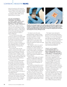
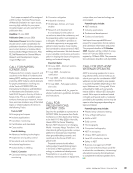
A total of nine steel samples, each measuring 12 in. × 4 in.
(30.5 cm × 10.2 cm) were prepared for corrosion inspection
using the robotic ECA setup. The samples included three
distinct geometries: one flat, four concave, and four convex, as
shown in Figure 3. These shapes were achieved using a sheet
roller, with curvatures designed according to corrosion stan-
dards detailed in Table 1. After shaping, the samples underwent
a seven-day salt spray corrosion process in accordance with
ASTM B117-03 (ASTM 2003). To create a calibration area for the
ECA, the bottom inch (2.54 cm) of each sample was treated
with a corrosion inhibitor however, some corrosion leached
into this section. Residual rust was removed using a soaking
solution.
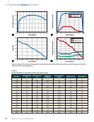
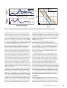
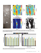
Comparison of Processed ECA Data with Microscope
Depth Profiling
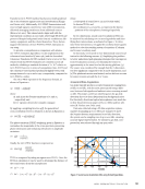
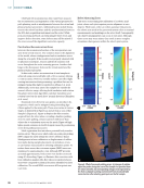
Ground truth volumetric data of surface corrosion were
obtained using a high-resolution digital microscope for
comparison with the ECA data. To locate the defects,
2D cross-correlation was applied, in which the microscope
data was searched across the ECA data. The best matching
pattern was indicated by the maximum correlation value
between the two sets. The patterns from ECA voltages cor-
related well with the depths of the microscope data.
Challenges in Robotic ECA Inspection of Curved
Samples
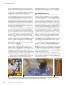
Detecting fine surface or underpaint corrosion defects (e.g.,
50 µm deep) on curved metallic surfaces using robotic arms
is challenging due to strict liftoff, tilt, and thermal stability
requirements for the ECA probe. For example, ECT typically
necessitates maintaining a close and constant liftoff (e.g.,
1 mm) between the coil probe and the metallic surface. Small
liftoff ensures a noncontact testing method, maximizing the
induction of eddy currents and achieving a high signal-to-
noise ratio (SNR) for the measurements. Additionally, surface
corrosion detection often requires sensor coils to operate at
excitation frequencies in the MHz range. As a result, probe
misalignment and temperature fluctuations can introduce
errors during the scanning process, affecting both defect
detection and the accurate quantification of defect depth.
This section explores the challenges faced during robotic ECT
and presents typical experimental images obtained using the
proposed robotic NDE system with computer vision.
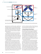
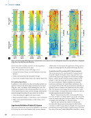
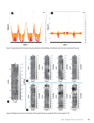
Effect of Inconsistent Probe Liftoff and Tilt on ECA
Measurements
Inconsistent liftoff typically introduces low spatial frequency
trends that overlap with defect indications, complicating image
processing and defect detection. Robotic manipulators can also
introduce inconsistent sensor tilt, affecting the distribution of
the excitation magnetic field from the coil sensor. For the rigid
and linear array probe, orientation errors affect each coil as a
body transformation, with coils at the edges of the array having
a different liftoff compared to the coils in its center. Improper
liftoff and/or tilt of the ECA probe can not only disrupt mea-
surements but also cause collisions with the test part, poten-
tially leading to immediate damage to the probe or long-term
degradation if dragged over rough surfaces.
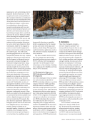
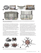
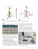
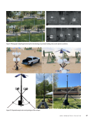
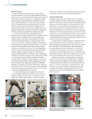
B1 B2 B3 B4 C1 C2 C3 C4 A
Figure 3. Steel samples with corrosion damage: (a) flat sample A (b) concave samples B1–B4 (c) convex samples C1–C4.
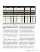
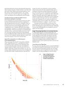
TA B L E 1
Curvatures of test samples with corrosion damage
Sample A B1 B2 B3 B4 C1 C2 C3 C4
Curvature k (1/m) 0.000 0.304 0.397 0.527 0.842 0.304 0.451 0.528 0.842
A P R I L 2 0 2 5 • M AT E R I A L S E V A L U AT I O N 65
A total of nine steel samples, each measuring 12 in. × 4 in.
(30.5 cm × 10.2 cm) were prepared for corrosion inspection
using the robotic ECA setup. The samples included three
distinct geometries: one flat, four concave, and four convex, as
shown in Figure 3. These shapes were achieved using a sheet
roller, with curvatures designed according to corrosion stan-
dards detailed in Table 1. After shaping, the samples underwent
a seven-day salt spray corrosion process in accordance with
ASTM B117-03 (ASTM 2003). To create a calibration area for the
ECA, the bottom inch (2.54 cm) of each sample was treated
with a corrosion inhibitor however, some corrosion leached
into this section. Residual rust was removed using a soaking
solution.
Comparison of Processed ECA Data with Microscope
Depth Profiling
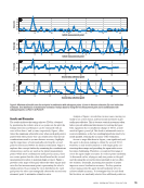
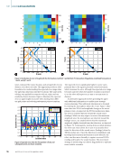
Ground truth volumetric data of surface corrosion were
obtained using a high-resolution digital microscope for
comparison with the ECA data. To locate the defects,
2D cross-correlation was applied, in which the microscope
data was searched across the ECA data. The best matching
pattern was indicated by the maximum correlation value
between the two sets. The patterns from ECA voltages cor-
related well with the depths of the microscope data.
Challenges in Robotic ECA Inspection of Curved
Samples
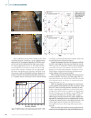
Detecting fine surface or underpaint corrosion defects (e.g.,
50 µm deep) on curved metallic surfaces using robotic arms
is challenging due to strict liftoff, tilt, and thermal stability
requirements for the ECA probe. For example, ECT typically
necessitates maintaining a close and constant liftoff (e.g.,
1 mm) between the coil probe and the metallic surface. Small
liftoff ensures a noncontact testing method, maximizing the
induction of eddy currents and achieving a high signal-to-
noise ratio (SNR) for the measurements. Additionally, surface
corrosion detection often requires sensor coils to operate at
excitation frequencies in the MHz range. As a result, probe
misalignment and temperature fluctuations can introduce
errors during the scanning process, affecting both defect
detection and the accurate quantification of defect depth.
This section explores the challenges faced during robotic ECT
and presents typical experimental images obtained using the
proposed robotic NDE system with computer vision.
Effect of Inconsistent Probe Liftoff and Tilt on ECA
Measurements
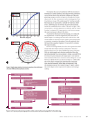
Inconsistent liftoff typically introduces low spatial frequency
trends that overlap with defect indications, complicating image
processing and defect detection. Robotic manipulators can also
introduce inconsistent sensor tilt, affecting the distribution of
the excitation magnetic field from the coil sensor. For the rigid
and linear array probe, orientation errors affect each coil as a
body transformation, with coils at the edges of the array having
a different liftoff compared to the coils in its center. Improper
liftoff and/or tilt of the ECA probe can not only disrupt mea-
surements but also cause collisions with the test part, poten-
tially leading to immediate damage to the probe or long-term
degradation if dragged over rough surfaces.
B1 B2 B3 B4 C1 C2 C3 C4 A
Figure 3. Steel samples with corrosion damage: (a) flat sample A (b) concave samples B1–B4 (c) convex samples C1–C4.
TA B L E 1
Curvatures of test samples with corrosion damage
Sample A B1 B2 B3 B4 C1 C2 C3 C4
Curvature k (1/m) 0.000 0.304 0.397 0.527 0.842 0.304 0.451 0.528 0.842
A P R I L 2 0 2 5 • M AT E R I A L S E V A L U AT I O N 65