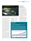
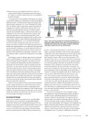
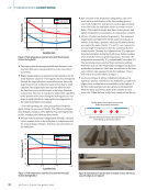
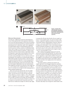
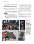
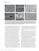
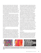
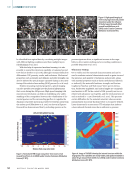
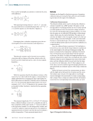
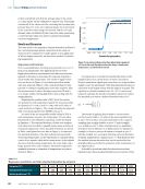
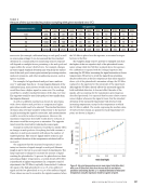
Here, nearby wavelengths are selected, to minimize the emis- sivity difference: (2) I(! 2 ,T) I(! 1 ,T) = ! 1 !2 " # & $5 % ’ e hc !1 kBT 1 e hc ! 2 k B T 1 With typical processing values (T = 1900 °C, λ ≈ 500 nm), the exponential term is considerably larger than 1 (ehc/λkBT ~ e7 ب"1) and the equation can be reduced to Equation 3: (3) I 2 ,T) ( I 1 ,T) ( = 1 2 ! " % #5 $ & e hc 1 kBT e hc 2 k B T Rearranging this to calculate temperature given the two wavelengths and recorded intensities yields Equation 4: (4) T = hc(" 2 "1) " 2 " 1 ln+ I#" 2 ,T% I#" 1 ,T% !, 2 #" $"1& %5 . ’ ( + ) * - - The physical constants can be factored out to produce a function with two degrees of freedom, which can be cali- brated to predict temperature given a ratio of sensor signals, Equation 5: (5) T = A ln) B I 1 ,T# ! I 2 ,T# ! % & ) ) ’ ( * * * While the equations describe the radiance/exitance of the source (I[λ,T]), it also holds for the signal, S, measured by two similar photodetectors occupying the same optical path. For linear photodetectors, filtered to relatively narrow wavebands (Δλ ا λ0), the measured signal is proportional to the source emittance: S0(T) ∝ I(λ0,T). In Equation 6, the constant of pro- portionality is either canceled or absorbed by the regression variable B: (6) T = A ln B S 1!T" S 2!T" $ % ( ( ( & ’ ) ) ) The measured signal ratio R(T) = S1(T)/S2(T). If T is known from a calibrated radiance source set to a specific set point Ti, then a regression model can be made: Ti = f (Ri,A,B), where Ti is the dependent variable, Ri is the independent variable, and A and B are unknown regression parameters. If a satisfactory regression function is found, it can then be used to evaluate a relative temperature, T, from measured signal ratio, R. Methods Methods are developed for the physics process of acquiring calibration data, processing the data collected, and normaliz- ing the data over the span of the build plate. Calibration Measurements The dual photodiode system used to develop the calibration scheme is installed on a LPBF machine. The gains on both the high and low wavelength sensors are set to ensure that the recorded signals are below the saturation voltage and above the noise floor during typical processing conditions. To ensure this, the gains are set while the LPBF machine is fabricating a square, which spans the entire build plate. The gains are set such that the higher of the two signals averages 75 of the sat- uration voltage across the build plate. At the end of the build, the laser is commanded to go to the center of the build plate, so that the galvanometer mirrors are focused for calibration on a central source. Next, the calibrated lamp is positioned. The build plate is lowered by 45 mm, such that the lamp’s filament is positioned at the same height as the melt pool during processing. The lamp is contained in the temperature calibration block such that it is horizontal and vertically aligned with the aperture on the top of the block. The high wavelength photodetector is removed, along with the optics tube, and replaced with a HeNe USB laser, which is used to illuminate the center of the build plate, and the calibration block is moved such that the lamp is centered on the build plate. After XY block alignment, the HeNe laser is removed and the high wavelength photodetector and optical tube are returned. A photo of the setup is shown in Figure 2. Before the lamp is powered on, measurements are taken with the lights turned off inside the 3D printer and the room. The median value of each of the high and low wavelength sensors with lights off is measured to be their corresponding dark voltages. These voltages are subtracted from all measure- ments from the corresponding sensors before they are used Figure 2. Photograph of calibration setup. ME | MELTPOOLMONITORING 66 M A T E R I A L S E V A L U A T I O N • A P R I L 2 0 2 2

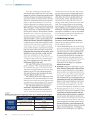
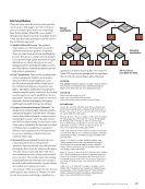
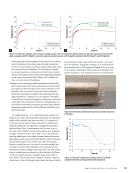
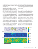
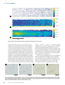
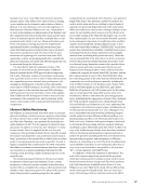
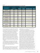
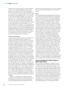
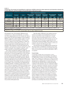
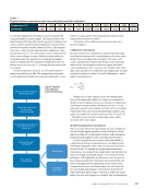
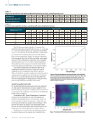
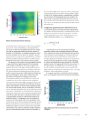
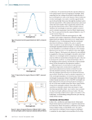
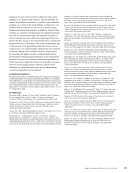
to calculate temperature. The lamp is current controlled by a programmable DC power supply. The lamp had been cali- brated using a NIST-traceable transfer pyrometer (Gibson et al. 1998) to achieve predetermined temperature set points when powered at a specific current, shown in Table 1. The tempera- ture is set to each set point and allowed to stabilize for 1 min, starting from 1300 °C. An oscilloscope is used to monitor both of the sensor voltages to ensure that they remain within the acceptable range. The aperture is set such that the higher sensor is reading 85 of its saturation voltage when the cali- bration source is set to 2300 °C, ensuring that the sensors will not saturate. At each temperature set point, 5 s of the photodetector signal is recorded at 200 kHz. The temperature is increased to each progressively higher set point and stabilized for 1 min before a 5 s data capture. The amperage set points for each temperature are shown in Table 1. A flowchart of the calibration measurement process is shown in Figure 3. Calibration Calculations Because both detector channels are acquired synchronously, each element corresponds to measurement at the same point in time. For each temperature set point Ti, the ratio, S1(T)/ S2(T), is calculated by elementwise division of the timeseries high and low wavelength photodetector signals after dark current subtraction, Ri(t) = S1(t)/S2(t). The median value of the time series ratio Ri(t) is recorded for each temperature set point and used to regress to values of A and B in Equation 7, which follows from Equation 6: (7) T i = A ln$ B Ri ! " # % Within each 5 s data capture of Ri(t), the standard devi- ation of the temporally middle 400 values was calculated to identify trends in signal variation as a function of temperature. Assuming a constant random distribution of noise, ˜, in the otherwise constant sensor signals S1(T) and S2(T) at a constant temperature, the noise is proportionally larger, relative to the signal. As a result, the variance in the ratio S(λ1,T) + ˜/S(λ2,T) + ˜ should increase with decreasing temperature, which decreases with sensor signal. Spatial Normalization Calculations There are many effects that may change the ratio of high and low wavelength signals spatially over the build plate, includ- ing but not limited to path length variation, angle-dependent transmission through the optics, and spherical aberration. It can be argued that the variation can be described as a proportional change in transmission in each high and low wavelength separately, which varies as a function of position and not in time. To quantify the proportional reduction in transmission, it is assumed that temperature, and therefore the ratio of low/high wavelength signals, is a constant across the build plate. Full build plates are fabricated once the process has reached a steady state, four layers are recorded. The raw data for the high and low signals from each of these layers is rastered into 50 μm resolution images. For each layer, the low wavelength signal image is elementwise divided by the high wavelength signal image, to produce a single ratio signal image. The four ratio images are averaged. The averaged image Center the laser focus on the center of the build plate Drop build plate by 45 mm, then place box in the center of it Record data with the bulb off Let stabilize for 1 min Prepare a data set Process one layer and set the detector gains Turn lamp to next set point Record data Figure 3. Flowchart of the calibration measurement process. T A B L E 1 Representative temperature and current set points used for calibration Temperature (°C) 1300 1400 1500 1600 1700 1800 1900 2000 2100 2200 2300 Current (A) 7.08 7.61 8.21 8.9 9.64 10.44 11.27 12.18 13.13 14.11 15.14 A P R I L 2 0 2 2 • M A T E R I A L S E V A L U A T I O N 67