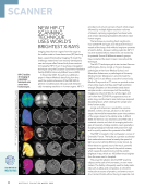
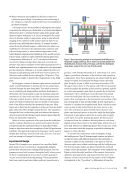
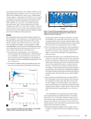
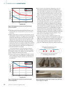
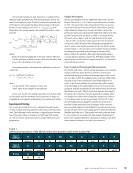
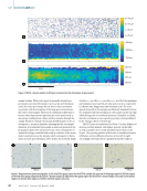
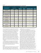
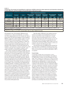
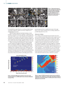
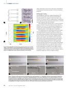
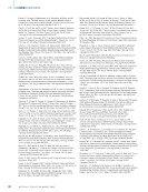
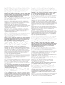
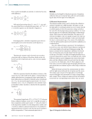
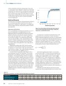
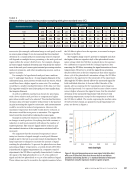
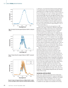
is then normalized such that the average value in the center 2 × 2 mm square on the build plate is equal to one. This image contains all of the values used for correcting the incoming tem- perature data. For every raw temporal datum, the nearest pixel in the correction value image was located, and the raw ratio datum’s value was divided by that correction value, producing a corrected ratio which was used to calculate the spatially corrected temperature. Results and Discussion The data are fit to the regression formula derived from Planck’s law, and temporal and spatial variation from the sensor is characterized. Comparison is made against in situ application of Wein’s displacement law, an alternative method of calculat- ing temperature. Regression and Variation Prior to standardization, the lamp was powered on to 1700 °C from room temperature. The signal from the low wave- length photodetector was measured over time as power was applied to the lamp to determine the timescale required to reach steady-state temperature. The results of signal versus time are shown in Figure 3. It was determined that steady state was achieved within 2 s. The 1 min dwell time for tem- perature to stabilize is significantly more than required. After this measurement is taken, the lamp is powered off until it is no longer visibly emitting light before proceeding with the standardization. Regressing the median value of Ri(t) (over the central 400 points) for each temperature against the set points yields an equation of A = 618.75 and B = 0.681, with an R2 value of 0.996, as shown in Figure 4. The model estimates the setpoints with a root mean square error (RMSE) of 19.42 °C. For each of the 400 temporally middle values of Ri(t) at each temperature set point, the temperature T(t) was calcu- lated based on the calibration regression model developed in Equation 7. The standard deviation of these 400 tempera- ture values was recorded to quantify sensor noise in terms of measured temperature. These standard deviations are shown in Table 2 and plotted as error bars in Figure 4. As expected, the standard deviation of the data collected increases with decreasing temperature, as the temperature is calculated from a ratio of two signals, which both contain noise. As the signals decrease with decreasing temperature, the noise makes up a larger portion of the ratio’s variance. Measured temperature standard deviation as a function of temperature set point is shown in Table 2. It is important to note that the standard deviation of the sampled data is not a good metric of sensor uncertainty. Because anomalous signals span more than one temporal data sample (5 μs), the uncertainty of the dual photodiode sensor is a function of the length of time that the signal is acquired. The equation to calculate standard error, SE = σ/√n, can be rear- ranged to calculate the number of samples required to reduce the standard error below a defined threshold value of SE: (8) n = ceiling ! #2 , % &"SE$ ) )* ’ ( + + The results of applying this formula to various values can be found in Table 3. To achieve the same standard error as 2300 °C but at other set point temperatures, the required sampling time roughly doubles at 2000 °C and is roughly 100× as high at 1300 °C. Here, standard error is a qualitative descriptor of how difficult it is to differentiate two signals. For example, to detect a process deviation in a signal at 1300 °C will take roughly 100× as long as detecting a process deviation of similar magnitude in a signal at 2300 °C. This illustrates that the quickest process deviation that can be resolved by this dual-photodetector method is a function of the temperature of the signal’s source. It should be noted that while the photodetectors have inherent noise, these standard deviations are a function of the 0.00 0.25 0.50 0.75 1.00 1.25 1.50 1.75 2.00 0.25 0.20 0.15 0.10 0.05 0.00 Seconds after powered on Figure 4. Low sensor voltage versus time when lamp is powered on. Due to the small thermal inertia of the lamp, a steady-state temperature is reached within seconds. T A B L E 2 Regression prediction and data standard deviation by set point Set point (°C) 1300 1400 1500 1600 1700 1800 1900 2000 2100 2200 2300 Standard deviation (°C) 734 382 225 190 148 130 109 104 87.8 77.5 73.0 Model prediction (°C) 1295 1361 1547 1603 1688 1803 1915 1998 2090 2206 2290 ME | MELTPOOLMONITORING 68 M A T E R I A L S E V A L U A T I O N • A P R I L 2 0 2 2 Low sensor voltage

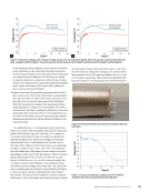
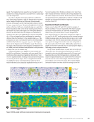
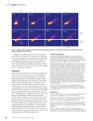
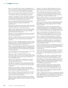
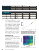
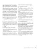
source size (for example, calibration lamp or melt pool) as well as sensor gain settings. It can be reasoned that the standard deviation of a coaxial melt pool monitoring sensor’s response will depend on multiple factors pertaining to the melt pool and region within the sensor’s field of view. For example, changes in sensor signal standard deviation may stem from the surface area of the melt pool, sensor gain/material processing window, melt pool emissivity, and other incandescing sources, such as spatter or plume. For example, if a hypothetical melt pool was a uniform 1300 °C and larger than the 2 × 8 mm tungsten filament of the calibration lamp, more photons would reach the sensor, which would then have a higher signal-to-noise ratio. The readings would have a smaller standard deviation of the data over time. The opposite would be true if the melt pool was smaller than the tungsten filament. As well, if a different material was chosen for processing with a lower relative melt pool size or temperatures, higher gain values would need to be selected. The standard deviation of sensor data over time would be reduced due to the increase in gain increasing the signal-to-noise ratio, and measurements could be recorded at reduced temperatures. However, the maximum temperature detectable would also be reduced, as the sensor would be more prone to saturation. The opposite trend would be observed for reducing the sensor gain. Changes in melt pool emissivity would have a similar effect as changes in melt pool size. Everything else held constant, a reduction in melt pool emissivity will reduce the number of emitted photons. The sensors’ signals will be reduced, and the standard deviation of the temperature calculated will be increased. The argument that the measured temperature’s uncer- tainty is a function of signal strength or melt pool/filament length is put to the test in a second round of experiments. The lamp’s aperture is enlarged to increase the amount of signal reaching the photodiodes. To prevent the photodetectors from saturating at higher temperatures, a neutral density (ND) filter is introduced at higher temperatures. In a separate round of experiments, the ND filter is optically characterized: it reduces the signal of the high photodiode to 13.71 of its unfiltered signal and the low photodiode to 10.57 of its unfiltered signal. These values are used to normalize the signals measured when the ND filter is placed over the aperture, to account for imper- fections in the filter. The tungsten lamp source’s aperture is enlarged such that the higher of the two signals is 85 of the photodiode’s satu- ration voltage while the ND filter is placed above the aperture. The calibration is repeated with the enlarged aperture after removing the ND filter, increasing the signal intensities at lower temperatures. However, to avoid the signal from saturating the photodetectors at the first temperature that either signal is above 75 of the photodiode’s saturation voltage, the ND filter is placed on the aperture for the remainder of the experiment. Although the ND filter directly affects the measured signal for both individual detectors, it does not affect the ratio of the signals, after accounting for the transmission percentages as described previously. It is expected that because relative sensor noise is higher whenever the signal is lower, that the standard deviation of the measured temperature will decrease with increasing temperature, except for the temperature at which the ND filter is added. The results, regressing the median value of Ri(t) (over the central 400 points) for each temperature set point, are shown in Figure 5. 2250 2000 1750 1500 1250 1000 750 500 Ratio (low/high) 0.42 0.44 0.46 0.48 0.50 0.52 Figure 5. Set point temperature versus mean signal ratio (blue dots) with curve fit (blue line). Note that the error bars do not indicate prediction uncertainty, but the ± 1σ standard deviation of measured temperature using the regression model at a given set point. T A B L E 3 Amount of time (μs) needed to produce sampling with given standard error (°C) Standard error (°C) Set point (°C) 1300 1400 1500 1600 1700 1800 1900 2000 2100 2200 2300 100 270 75 30 20 15 10 10 10 5 5 5 75 480 130 45 35 20 20 15 10 10 10 5 50 1080 295 105 75 45 35 25 25 20 15 15 25 4315 1170 405 290 180 140 100 90 65 50 45 10 26 940 7300 2535 1805 1100 845 595 545 390 305 270 A P R I L 2 0 2 2 • M A T E R I A L S E V A L U A T I O N 69 Temperature (ºC)