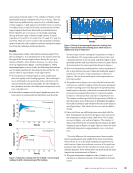
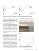
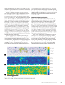
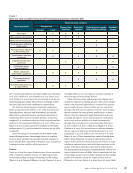
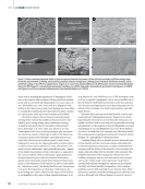
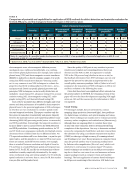
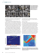
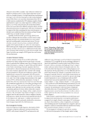
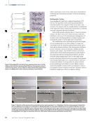
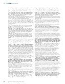
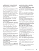
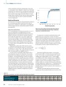
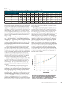
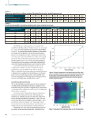
The ND filter was added at the 1800 °C set point. The model fits to this data with an R2 value of 0.996, A = 447.52, and B = 1.0523. The model estimates the set points with an RMSE of 19.70 °C. As expected, the standard deviations of this model are overall lower compared to the previous model, particu- larly at lower temperatures. There is an increase in deviation at the data point where the ND filter was added, as the signal decreased. The model predicts temperature with a standard deviation which is 1.3 to 6.1 of the set point temperature. The predictions of the regression model and standard devia- tions of the temperature predictions can be found in Table 4. In a similar construction as the previous data set, the sampling time needed to produce a sample with a given standard error was calculated for this data set, shown in Table 5. It should be noted that neither the standard deviations or durations for a standard error for this data set or the prior data set are necessarily characteristic of the standard devia- tions and sampling periods during AM processing. As stated, there are other inputs that will affect these values. Spatial Normalization Results For the full build plate measurements, the data is sampled at 200 kHz and the standardization formula is applied to each individual data point to predict a temperature for that location. A scatterplot of the temperature values from the full build plate build is shown in Figure 6. As described in the “Spatial Normalization Calculations” section, for every data point, the ratio of the signals was divided by the spatially nearest correction value, which was used to calculate an adjusted temperature. A plot of the cor- rected values from the ratio image is shown in Figure 7. Note that the ratio values are similar to the temperature values because the function that relates them is nearly linear. A scat- terplot of the corrected temperatures is found in Figure 8. Qualitatively, it is clear that this standardization reduced the spatial variations in the original data. Quantitively, the 200 150 100 50 3000 2500 2000 1500 1000 X position (mm) 25 50 75 100 125 150 175 200 225 Figure 7. Scatterplot of the temperature data over the full build plate. 2200 2000 1800 1600 1400 1200 Ratio (low/high) 0.74 0.76 0.78 0.80 0.82 0.84 0.86 Figure 6. Set point temperature versus mean signal ratio (blue dots) with curve fit (blue line) for the neutral density experiment. Note that the error bars do not indicate prediction uncertainty, but the ± 1σ standard deviation of measured temperature using the regression model at a given set point. T A B L E 4 Regression prediction and data standard deviation by set point, variable aperture run Set point (°C) 1300 1400 1500 1600 1700 1800 1900 2000 2100 2200 2300 Standard deviation (°C) 79.7 49.2 34.4 29.0 22.7 69.0 58.3 52.7 44.4 40.0 34.6 Model prediction (°C) 1352 1389 1477 1591 1703 1800 1891 1984 2095 2195 2321 T A B L E 5 Duration (μs) needed to produce sampling with given standard error (μs) Standard error (°C) Set point (°C) 1300 1400 1500 1600 1700 1800 1900 2000 2100 2200 2300 100 5 5 5 5 5 5 5 5 5 5 5 75 10 5 5 5 5 5 5 5 5 5 5 50 15 5 5 5 5 10 10 10 5 5 5 25 55 20 10 10 5 40 30 25 20 15 10 10 320 125 60 45 30 240 175 140 100 80 60 ME | MELTPOOLMONITORING 70 M A T E R I A L S E V A L U A T I O N • A P R I L 2 0 2 2 Y position (mm) Temperature (ºC) Temperature (ºC)

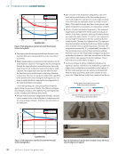
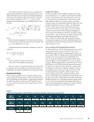
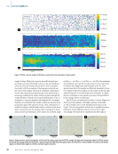
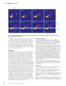
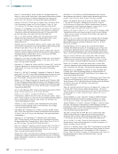
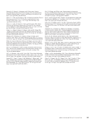
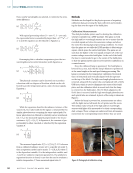
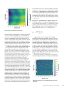
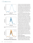
standard deviation of temperatures in the noncorrected data set is 109 °C. In the corrected data set, the standard devia- tion is 32.8 °C. However, this adjustment makes the assump- tion that the temperature should not vary as a function of position on the build plate. In using this assumption, all real position-dependent process effects are masked. A superior approach may be to improve the optical hardware, such that position-dependent optical transmission is reduced, using knowledge of the source of the position-variation pattern. The presence of the patterns can be reasonably attributed to optical interference patterns produced by the partially coherent light emanating from the melt pool/plume com- bination. The source of the light is always related to that of the laser, which provides the power to melt the powder bed. The infrared radiation is transformed in and near the melt pool by various processes into visible radiation, which propa- gates back through the optical system of the printer. The procedure for transformation of high-power, focused, near-infrared radiation proceeds as follows. A melt pool is established by the focused radiation having considerable vapor pressure of the printed alloy constituents. These metal vapor atomic species are partially ionized through the photo- electric effect driven by the focused laser’s high electric field. The electrons and metallic ions are accelerated by the laser’s electric field and collisionally excite the neutral atoms to states above those established by the thermally induced Boltzmann distribution characteristic of the somewhat superheated melt pool. These excited states due to collisional excitation have a high probability of radiation with lifetimes usually in the nanosecond range. A competing process, de-excitation by collisions with cooler species, has a lower probability as the system density is low. In the meantime, the thermally excited Boltzmann distribution of metal quantum states contributes background radiation of a lesser amount at the wavelength’s characteristic of the respective materials. Another important process is the nonlinear optical production of harmonics of the near-infrared high-power melt laser with the metal vapor components acting as the nonlinear optical medium. Finally, because of the strongly nonlinear, nonequilibrium conditions that are present, the emerging light spectrum (visible in the spectroscopy of the plume) has partial coherence, driven by the melt laser, which causes the interference patterns. In prin- ciple, this can be eliminated by depolarizing the light entering the optical train. Comparison Against Alternative Method: Wien’s Law An alternative approach to bichromatic Planck thermometry is to measure the entire spectrum of a radiating source. Wien’s displacement law indicates that the temperature of a black- body (or graybody) source can be calculated from the wave- length of maximum radiance (λmax) using Equation 9: (9) T = 2.898!10 3 m!K " max A spectrometer is used to measure the wavelength- dependent emission from the tungsten filament at the same seven calibration set points. In one experiment, the spectrom- eter was placed on axis, replacing one of the photodetectors, while the tungsten lamp remained in the same position as described previously. In another experiment, the spectrometer was placed off axis, directly in front of the tungsten filament, so that the emitted light did not pass through all of the LPBF machine’s optics. For temperatures between 1300 and 1900 °C, the expected peak wavelength values are between 1333 and 1842 nm. However, the spectrometer is most sensitive in the visible range the off-axis spectra of the bulb at 1600 °C is found in Figure 9, with a peak radiance at 716 nm. In a separate experiment, each element of the machine’s optics were separately characterized for spectral transmittance 200 150 100 50 1.2 1.1 1.0 0.9 0.8 0.7 0.6 X position (mm) 25 50 75 100 125 150 175 200 225 Figure 8. Correction values from the ratio image. 200 150 100 50 2100 2000 1900 1800 1700 1600 1500 1400 X position (mm) 25 50 75 100 125 150 175 200 225 Figure 9. Scatterplot of the corrected temperature data over the full build plate. A P R I L 2 0 2 2 • M A T E R I A L S E V A L U A T I O N 71 Y position (mm) Y position (mm) Temperature (ºC) Temperature (ºC)