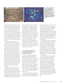
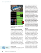
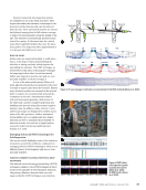
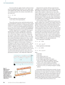
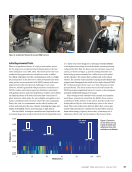
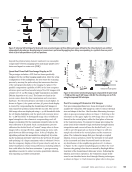
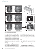
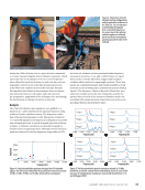
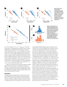
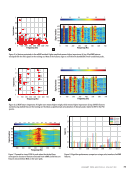
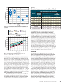
filtered and then subtracted from the original slice to flatten
the noise “phantoms.” From the sample slice in the vertical
plane, the smoothing process does not change the intensity
of the main lobe response. Since the noise floor is identi-
fied in each transverse plane, the volumetric intensity map
can finally be projected onto the transverse plane such that
the high intensity pixels are coherently added up, while the
lower intensity pixels remain at their intensity levels. Shown
in Figure 7d, after converting the grayscale image to decibel
levels, the example transverse defect is finally identified with a
high contrast.
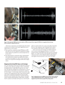
At this point of the processing, it is necessary to isolate the
flaw from the background image. The critical step to highlight
the edge of the flaw is to apply a decibel level threshold and
convert the intensity map into a binary map. Typically, the
threshold is chosen as –15 dB for a ~30 dB dynamic range SAF
image, but the value should be adaptive to various circum-
stances such as defect orientation, reflectivity, SNR, and so
forth. In this paper a dynamic threshold level is determined
through the following empirical equation: ​ ​
(3)​ Threshold =a +b *cos(​θ​defect​​)​ ​ +c *noise​
where
{a, b, c} are empirical constants calibrated from ground truth
results from known flaws,
θdefect is the incident angle of the acoustic beams on the flaw,
and
noise is the decibel level of the background phantom deter-
mined in the flattening process.
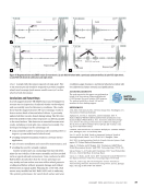
To find the incident angle θdefect, the algorithm first
approximates the tilted angle φ of the flaw using the initial 3D
ME
|
RAILROADS
10
20
60 70 80 90 100
30
40
Length y (mm)
10
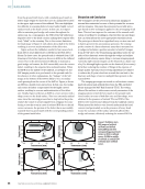
Vertical plane Transverse plane
Morphology
Filter
Binary
20
–20 –10 0
Horizontal plane
(x-y)
Defect
Artifact
Vertical plane
SAF image slices
(y-z)
Transverse plane
Final defect image
(x-z)
10 20
30
40
Transverse x (mm)
3D
10
20
60 70 80 90 100
30
40
Length y (mm)
10
20
–20 –10 0 10 20
30
40
Transverse x (mm)
10
20
–20 –10 0 10 20
30
40
Transverse x (mm)
10
20
–20 –10
Project to 2D
0 10 20
30
40
–10
0
–20
–30
Transverse x (mm)
3D
10
20
60 70 80 90 100
30
40
Length y (mm)
10
20
–20 –10 0 10 20
30
40
Transverse x (mm)
3D
x
z
y
Figure 7. Volumetric image post-processing flowchart.
56
M A T E R I A L S E V A L U A T I O N • J A N U A R Y 2 0 2 4
2401 ME January.indd 56 12/20/23 8:01 AM
Depth
z
(mm)
Depth
z
(mm)
Depth
z
(mm)
Depth
z
(mm)
Depth
z
(mm)
Depth
z
(mm)
Depth
z
(mm)
Depth
z
(mm)

visualization by projecting the 3D cluster on arbitrary inclined
transverse planes and finding the angle of the tentative plane
that results in the maximum area of the defect. The incident
angle is then computed by considering the geometric rela-
tionship between the broadside of the refracted acoustic
beams and the defect inclination φ. As an example, consider
a 30 dB dynamic range tomography of a sample transverse
defect with an estimated inclination φ =20°. The resulting
incident angle θdefect using the 55° shear wedge is 15°. A rea-
sonable set of empirical constants is therefore a =1.5, b =
–2, and c =0.5 to obtain a threshold of –15.4 dB. When the
incident angle is small, it is appropriate to increase the search
range in the decibel levels since the defect gives a good
reflection to the array (higher contrast image), which results
in a negative value of b. The additional consideration of
noise level gives a second chance of energy level adjustment
according to the image SNR.
The final binary defect image is shown in Figure 7e.
Typically, for a single flaw present in the scanner area, a
good SNR in SAF imaging results in only one cluster of pixels.
However, as in the case of Figure 7e, a less than ideal SNR
may result in artifacts that still need to be segmented out
before the final estimation of the flaw size. For this purpose,
the algorithm further segments the 3D point cloud using
the k-means clustering algorithm by calculating a minimum
Euclidean distance between pixels to form identified clusters.
The minimum Euclidean distance is set to 1.4 mm (S-wave
resolution in steel) to differentiate between different clusters
of pixels, and the clusters are arranged in descending order
per area. To account for cases of multiple separate flaws
within the same scanned area, the GUI includes the possi-
bility to investigate each individual cluster if the secondary
clusters are worthy of attention.
Experimental Results
Validation of the rail flaw SAF imaging prototype was per-
formed on flawed rail sections from the FRA defect library
managed by MxV Rail. Some of the test sections con-
tained natural rail defects, while others contained artificial
defects. Following the scanning by the prototype at UCSD
Experimental Mechanics &NDE Laboratory, each test rail
section with natural defects was broken by MxV Rail person-
nel to establish the “ground truth” from visual observation of
the flaws. Following the initial validation, some parameters in
the SAF post-processing algorithms were optimized to better
match the ground truth.
Figure 8 shows the final images obtained by the SAF
imaging prototype for three natural defects from three FRA
rail sections compared to the corresponding ground truth
pictures after the rail breaks. Figure 8a shows the case of a
natural transverse defect (TD) in a weld. In this case, the
size and shape of the defect are perfectly imaged by the SAF
system, with a size error as low as –2.3%. This example, there-
fore, shows an ideal case of a strong reflector (large SNR of
the ultrasonic reflections) and located in a region that allowed
good contact between the wedge and the rail surface during
manual scanning. Figure 8b shows the case of a void defect
in the welded region of another rail section. The ground truth
picture shows a clear indication of the void with the oxidized
boundary. However, compared to the first case of the TD,
the void defect is a slightly weaker reflector of ultrasound. In
the raw SAF images for this case, the noise level is as high as
–25 dB, and some areas of the reflection from the weld may be
mistaken for the defect in the initial 3D point cloud display.
However, as shown in Figure 8b, the post-processing routine
described in the previous section successfully isolates the
void reflector with a final defect area estimation only differing
SAF image
Ground truth
ROI
0
10
20
–40 –20 0 20 40
30
40
50
Transverse x (mm)
0
10
20
–40 –20 0 20 40
30
40
50
Transverse x (mm)
0
10
20
–40 –20 0 20 40
30
40
50
Transverse x (mm)
Figure 8. Validation tests. SAF images of natural rail flaws and their corresponding ground truth pictures: (a) a transverse defect in a weld (b) a void
in a weld and (c) a transverse defect in the railhead corner.
J A N U A R Y 2 0 2 4 • M A T E R I A L S E V A L U A T I O N 57
2401 ME January.indd 57 12/20/23 8:01 AM
Depth
z
(mm)
Depth
z
(mm)
Depth
z
(mm)