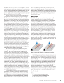
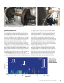
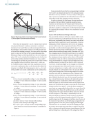
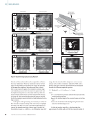
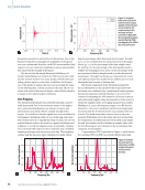
frequencies around 370 and 530 Hz, not shown here. Due to the
hammer being driven manually, the amplitudes of the spectra
were not constant and, therefore, each PSD was normalized with
respect to its own maximum amplitude to remove any potential
bias caused by the strength of the impact.
Not shown here but amply discussed in Belding et al.
(2023b) and Belding et al. (2023c), the PSD between the wired
and the wireless sensors were quite similar, with the latter pro-
viding a better signal-to-noise ratio. In addition, the frequen-
cies of the peaks on a given day were not necessarily the same
on the following day, or from one year to the next. This is con-
sistent with what is discussed in Figure 2 and is likely related to
a change in the rail’s boundary conditions.
Data Prepping
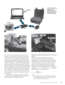
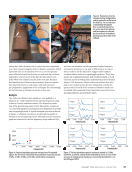
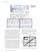
The instrumented hammer was operated manually, as previ-
ously mentioned. Due to the stochastic nature of the impact
force, min-max normalization was chosen to remove any
inherent bias associated with the variable strength of the
impact. It is noted here that the signals were not normalized by
the hammer’s maximum value, as one of the long-term objec-
tives of the project is to simplify the setup. As such, the use of a
regular hammer without the need for a signal conditioner and
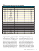
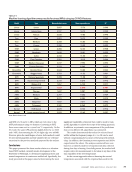
a digitizer to record the impulsive force is preferable. Datasets
were clustered with respect to the tie material, and a stratified
sampling technique was used across each day. This sampling
scheme split the data into train/validation/test splits, which
kept the percentage taken from each day the same. The split
35-15-50 was considered in the study presented in this paper,
where (35 +15) is the percentage of the data samples used
for training 15 is the percentage of the training data used to
validate the learning process and 50 is the percentage of the
never-presented-before samples used to predict the neutral
temperature. This split was chosen as it represents the worst-
case split out of previous studies by the authors due to it con-
taining the least amount of training data.
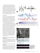
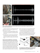
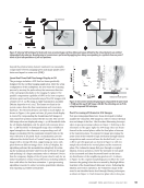
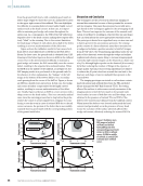
The lateral component of the vibration measured by
the accelerometers on the rail above the tie and above the
mid-span were combined into a single signal using frequency
domain decomposition (FDD) (Brincker et al. 2001). FDD
consists of computing the PSD matrix for all sensor locations
and performing singular value decomposition of the matrix to
obtain the singular values. Leveraging upon previous studies
(Belding et al. 2023), the frequency range 0–700 Hz and res-
olution of 0.1 Hz were considered, and the head temperature
measured with the K/J thermometer was considered for two
reasons. The head temperature may be closer to the tem-
perature distribution across the whole rail cross section than
the temperature recorded from the web located in the shade.
Second, the number and the timeline of samples taken with
the K/J thermometer were identical to the acceleration data,
easing the overall analysis.
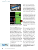
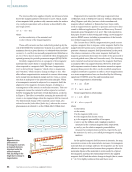
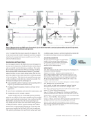
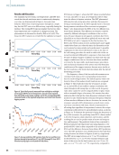
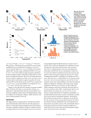
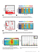
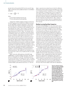
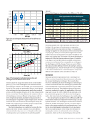
A representative FDD is provided in Figure 4, which shows
the combined PSD via FDD associated with the wired and
ME
|
RAILROADS
0
0
–0.5
–1
0.5
1
–0.05 0.05
Time (s)
0.1 0.15 0.2 0
0
0.2
0.4
0.6
0.8
1
200 400 600 800 1000
Frequency (Hz)
Lateral
Vertical
Figure 3. (a) typical
time series associated
with the lateral impact
applied at the mid-span
and recorded by the
accelerometer at the
mid-span on Day 1
(concrete) in May 2021
(b) corresponding power
spectral density (PSD)
overlapped to the PSD of
the vertical direction.
0
0.2
0.4
0.6
0.8
1
0
0
0.2
0.4
0.6
0.8
1
200 100 400 300 600 500 700
Frequency (Hz)
0 200 100 400 300 600 500 700
Frequency (Hz)
Figure 4. Example
of pooled spectral
information via FDD:
(a) lateral direction
and (b) vertical
direction.
70
M A T E R I A L S E V A L U A T I O N • J A N U A R Y 2 0 2 4
2401 ME January.indd 70 12/20/23 8:01 AM
Amplitude
(V)
PSD
amplitude
×
10–6
Normalized
amplitude
Normalized
amplitude

wireless sensor. The FDD encompassed the only input to the
models for feature extraction so we could remove any reliance
on temperature and strictly associate with RNT. Seven different
algorithms were considered: LR, decision trees, SVM, ensem-
bles, GPR, and ANN, as well as kernel approximation methods.
Alongside the base algorithms provided in MATLAB, varia-
tions in a few base parameters were also tested. These include
kernel type for GPRs and SVMs and number of hidden layers
for ANN. All the models in addition to their parameter varia-
tions are listed Table 1.
To compare the different algorithms, the input vector
consisted of the two full FDD amplitude directions, the corre-
sponding frequencies, and the temperature manually recorded
from the railhead probe at those excitations. The performance
of each model was determined by calculating the mean-
squared error (MSE) associated with the RNT: ​ ​
(3)​ MSE =​ 1
n ​ ​ ∑
i=1​
n ​ ​ ​
(​​ ​ Yi​​​ − ​ ˆ ​ ​ i​​​​ )​​​​
2​​​
where​​
Y​i​​​ is the ground truth RNT, ​ ​
ˆ ​ ​ i​​​​ is the neutral temperature predicted by the algorithm, and
n represents the number of total experimental
measurements.
This was chosen to penalize outliers during the training
procedure, which is accomplished by using the square term.
The RNT was chosen as the target instead of the stress due to
T A B L E 1
Types of machine learning algorithms tested with their variants
Model Type Note
Linear Linear Terms linear
Linear Interactions Terms interactions
Linear Robust Terms linear, robust
Tree Fine Minimum leaf size 4
Tree Medium Minimum leaf size 12
Tree Coarse Minimum leaf size 36
SVM Linear Linear kernel
SVM Quadratic Quadratic kernel
SVM Cubic Cubic kernel
SVM Fine Gaussian Gaussian kernel, kernel scale 6.6
SVM Medium Gaussian Gaussian kernel, kernel scale 26
SVM Coarse Gaussian Gaussian kernel, kernel scale 110
GPR Rational quadratic Rational quadratic kernel, constant basis
GPR Squared
exponential Squared exponential kernel, constant basis
GPR Matern 5/2 Matern 5/2 kernel, constant basis
GPR Exponential Exponential kernel, constant basis
Ensemble Boosted trees Minimum leaf size 8, 30 learners,
0.1 learning rate
Ensemble Bagged trees Minimum leaf size 8, 30 learners
ANN Narrow 1 layer, ReLU activation, 10 nodes
ANN Medium 1 layer, ReLU activation, 25 nodes
ANN Wide 1 layer, ReLU activation, 100 nodes
ANN Bilayered 2 layer, ReLU activation, 10 nodes each
ANN Trilayered 3 layer, ReLU activation, 10 nodes each
Kernel SVM kernel SVM kernel learner
Kernel Least-squares
kernel regression Least-squares kernel learner
J A N U A R Y 2 0 2 4 • M A T E R I A L S E V A L U A T I O N 71
2401 ME January.indd 71 12/20/23 8:01 AM