
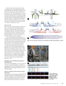
ties) among the tie spans between the measurement sites
vary, ranging from 0.23 to 0.3 m (9 to 12 in.). Approximately at
the midpoint between the two measurement locations, a rail
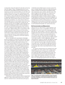
de-stressing procedure (rail cut) was applied. The rail cut was
applied on the fourth tie span toward the west direction from
the East location, as shown in Figure 1.
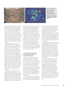
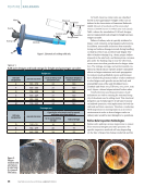
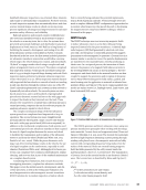
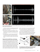
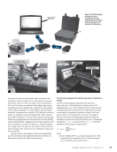
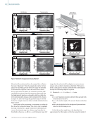
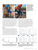
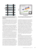
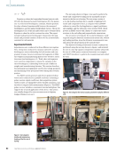
At both testing locations, the rail web was instrumented
with two sets of strain gauge modules (active set and spare
set) and temperature sensors, as shown in Figure 2. At each
location, the strain measurement system uses a four-leg full-
bridge gauge comprising two axial and two transverse (vertical)
strain gauges, the output of which is modified to account for
transverse strains owing to temperature and the Poisson effect
when a value of Poisson ratio (0.285 was used to represent rail
steel here) is input to the system, the output value from the
gauges is an equivalent axial strain value x This approach has
been well established in practice (Samavedam et al. 1986), and
values of x obtained with such systems have been shown to
well represent the axial stress state in the rail owing to confined
thermal expansion (Liu et al. 2018). For the remainder of this
paper, the compensated equivalent strain output x will simply
be referred to as axial strain or microstrain. Alongside the
strain gauge modules, one resistance temperature detector
(RTD) on each side of the rail at each location was installed for
monitoring the rail temperature. Together these sensors enable
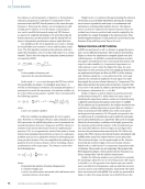
the rail RNT to be calculated using the formula:
(2) RNT =T − εx
α
where
εx is the equivalent axial strain,
α is the presumed linear thermal expansion coefficient 1.169
× 10–5/°C (6.5 × 10⁻⁶/°F), and
T is the rail temperature.
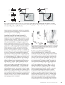
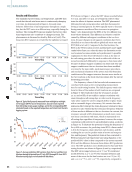
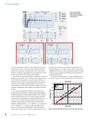
The rail temperature, axial strain, and RNT readings are
transmitted to a track-side solar-powered, stand-alone data
logging system. The entire measurement system was installed
and tested one day before the rail-cutting procedure. The
logging system has continuously reported the temperature,
strain, and RNT data every 15 min since it was installed.
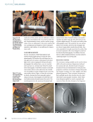
The rail-cutting procedure was conducted on the morning
of 31 July 2019. The cutting process released the rail stress
(tension) around the cut region and then the rail was pulled
and connected with a thermite weld to set the RNT to a
desired value. Because the strain and temperature measur-
ing system was deployed and operating before the rail cut
occurred, the equivalent axial strain and RNT of the system at
the two measurement locations can be accurately measured
moving forward. All reported strain and RNT are referenced by
the original cutting procedure, and no subsequent rail-cutting
procedure or other gauge calibration processes were carried
out. Although sensor systems are known to exhibit errors,
such as value drift, over the long term, in this case it is reason-
able to presume that the overall drift of the multisensor full-
bridge strain system will likely provide insignificant changes
with respect to the stress-state changes the system measures,
because the random drift of individual sensors within the
combined full-bridge system are likely to cancel each other out
over the two-year measurement period. To check for possible
drift problems, we switched from active to spare strain sensor
sets mounted nearby after over one year of measurement and
found no significant change in the strain readings.
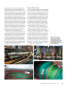
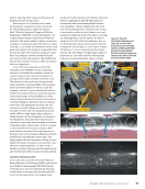
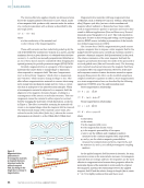
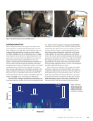
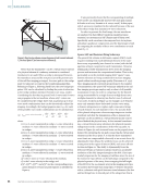
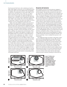
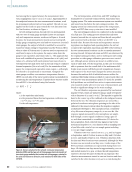
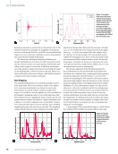
The rail vibration responses are generated by mechanical
impulse events, which are initiated using a small steel sphere
with a diameter of 12 mm (0.47 in.). The impulse is applied by
hand to the center top of the railhead at the midspan location
between the ties. The vibration responses are sensed by a
polarized condenser microphone pointing to the side of the
railhead at the same location where the impulse is applied,
as illustrated by Figure 3. The microphone has a sensitivity
of ±3 dB across a frequency range of 4 to 100 000 Hz. The
response signals measured by the microphone are ampli-
fied through a sensor signal conditioner using a gain of
10, and then transmitted to a multifunction I/O device for
data acquisition. Each collected time signal set up by the
mechanical impulse is 0.3 s in duration with a sampling rate
of 500 kHz with a total of 150 001 sample points including
10 000 pre-trigger samples.
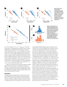
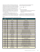
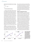
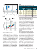
Vibration tests were carried out on 1, 5, 15, and 29 August,
19 September, and 18 October in 2019 29 May and 8 October
in 2020 and finally 16 June in 2021. Vibration data from both
the East and West locations were measured, although the West
location was not tested on 29 May 2020. A wide range of the
RNT and strain conditions are represented during these test
days. All vibration test days started at approximately 9:00 a.m.
and ended around 3:00 p.m. or when the rail temperature
started to decrease because of reduced sun exposure. The
vibration measurements started at one test location and then
switched to the other location every 40 to 60 min during the
ME
|
RAILROADS
RTD
Strain gauge modules
Figure 2. Sensors attached to the rail web: resistance temperature
detectors (RTD) and the two sets of strain gauges. Each set consists of
two strain gauge modules that contain two strain gauges, oriented in
the axial and transverse direction, each attached on both sides of the
rail web.
62
M A T E R I A L S E V A L U A T I O N • J A N U A R Y 2 0 2 4
2401 ME January.indd 62 12/20/23 8:01 AM
vary, ranging from 0.23 to 0.3 m (9 to 12 in.). Approximately at
the midpoint between the two measurement locations, a rail
de-stressing procedure (rail cut) was applied. The rail cut was
applied on the fourth tie span toward the west direction from
the East location, as shown in Figure 1.
At both testing locations, the rail web was instrumented
with two sets of strain gauge modules (active set and spare
set) and temperature sensors, as shown in Figure 2. At each
location, the strain measurement system uses a four-leg full-
bridge gauge comprising two axial and two transverse (vertical)
strain gauges, the output of which is modified to account for
transverse strains owing to temperature and the Poisson effect
when a value of Poisson ratio (0.285 was used to represent rail
steel here) is input to the system, the output value from the
gauges is an equivalent axial strain value x This approach has
been well established in practice (Samavedam et al. 1986), and
values of x obtained with such systems have been shown to
well represent the axial stress state in the rail owing to confined
thermal expansion (Liu et al. 2018). For the remainder of this
paper, the compensated equivalent strain output x will simply
be referred to as axial strain or microstrain. Alongside the
strain gauge modules, one resistance temperature detector
(RTD) on each side of the rail at each location was installed for
monitoring the rail temperature. Together these sensors enable
the rail RNT to be calculated using the formula:
(2) RNT =T − εx
α
where
εx is the equivalent axial strain,
α is the presumed linear thermal expansion coefficient 1.169
× 10–5/°C (6.5 × 10⁻⁶/°F), and
T is the rail temperature.
The rail temperature, axial strain, and RNT readings are
transmitted to a track-side solar-powered, stand-alone data
logging system. The entire measurement system was installed
and tested one day before the rail-cutting procedure. The
logging system has continuously reported the temperature,
strain, and RNT data every 15 min since it was installed.
The rail-cutting procedure was conducted on the morning
of 31 July 2019. The cutting process released the rail stress
(tension) around the cut region and then the rail was pulled
and connected with a thermite weld to set the RNT to a
desired value. Because the strain and temperature measur-
ing system was deployed and operating before the rail cut
occurred, the equivalent axial strain and RNT of the system at
the two measurement locations can be accurately measured
moving forward. All reported strain and RNT are referenced by
the original cutting procedure, and no subsequent rail-cutting
procedure or other gauge calibration processes were carried
out. Although sensor systems are known to exhibit errors,
such as value drift, over the long term, in this case it is reason-
able to presume that the overall drift of the multisensor full-
bridge strain system will likely provide insignificant changes
with respect to the stress-state changes the system measures,
because the random drift of individual sensors within the
combined full-bridge system are likely to cancel each other out
over the two-year measurement period. To check for possible
drift problems, we switched from active to spare strain sensor
sets mounted nearby after over one year of measurement and
found no significant change in the strain readings.
The rail vibration responses are generated by mechanical
impulse events, which are initiated using a small steel sphere
with a diameter of 12 mm (0.47 in.). The impulse is applied by
hand to the center top of the railhead at the midspan location
between the ties. The vibration responses are sensed by a
polarized condenser microphone pointing to the side of the
railhead at the same location where the impulse is applied,
as illustrated by Figure 3. The microphone has a sensitivity
of ±3 dB across a frequency range of 4 to 100 000 Hz. The
response signals measured by the microphone are ampli-
fied through a sensor signal conditioner using a gain of
10, and then transmitted to a multifunction I/O device for
data acquisition. Each collected time signal set up by the
mechanical impulse is 0.3 s in duration with a sampling rate
of 500 kHz with a total of 150 001 sample points including
10 000 pre-trigger samples.
Vibration tests were carried out on 1, 5, 15, and 29 August,
19 September, and 18 October in 2019 29 May and 8 October
in 2020 and finally 16 June in 2021. Vibration data from both
the East and West locations were measured, although the West
location was not tested on 29 May 2020. A wide range of the
RNT and strain conditions are represented during these test
days. All vibration test days started at approximately 9:00 a.m.
and ended around 3:00 p.m. or when the rail temperature
started to decrease because of reduced sun exposure. The
vibration measurements started at one test location and then
switched to the other location every 40 to 60 min during the
ME
|
RAILROADS
RTD
Strain gauge modules
Figure 2. Sensors attached to the rail web: resistance temperature
detectors (RTD) and the two sets of strain gauges. Each set consists of
two strain gauge modules that contain two strain gauges, oriented in
the axial and transverse direction, each attached on both sides of the
rail web.
62
M A T E R I A L S E V A L U A T I O N • J A N U A R Y 2 0 2 4
2401 ME January.indd 62 12/20/23 8:01 AM


