
the reliance on rail temperature in Equation 2. During feature
extraction, frequencies could then be constrained to those
associated with the RNT directly instead of the stress through
Equation 2. Removing the reliance on rail temperature addi-
tionally proves whether or not the impact of rail tempera-
ture can be modelled adequately using only PSD features
as opposed to explicitly providing it. It is noted here that for
feature extraction, models included only the lateral FDD as
input to demonstrate performance using a single direction.
The mRMR and the NCA algorithms were used to identify
the bandwidths most sensitive to stress and boundary condi-
tions. The first algorithm maximizes the relevance and mini-
mizes the redundancy of a set of data with respect to a certain
variable. This is done by using the maximum mutual informa-
tion quotient (MIQ):
(4) max
x ∈ Sc MIQx = max
x ∈ Sc
I(x, y) _
1
|S|
∑ z∈S I(x, z)
where
S is the number of features, and
I represents the mutual information.
In this study, S =700 to start because the PSD from which
the bandwidths are going to be identified spans from 0 to
700 Hz at 1 Hz frequency resolution. The mutual information I
measures how much the uncertainty of a random variable can
be reduced by knowing another variable. This is determined by
the following equation:
(5) I ( X, Z ) = ∑
i,j P(X = xi, Z = zj)log_______________ P(X = xi, Z = zj)
P(X = xi)P(Z = zj)
where
X and Z are random variables.
If the two variables are independent, I(X, Z) is equal to
zero. Therefore, to determine relevance and redundancy in the
PSD spectrums, the mRMR algorithm is used to maximize the
mutual information between a frequency and RNT whereas it
minimizes the mutual information between neighboring fre-
quencies. NCA is a nonparametric method that seeks to obtain
features that maximize the prediction accuracy of a regression
problem and acts as an alternative method to determining the
most prevalent features. This is accomplished by making use of
gradient descent to learn a distance metric by finding a linear
transformation of the input space. The distance metric takes
the following form:
(6) dw ( xi, xj ) = ∑
z=1
P wz 2 |xiz − xjz|
where
P represents the number of features (frequencies),
wz is feature weight, and
xiz and xjz are observations associated with said feature and a
random reference observation.
Weight vector w is optimized by approximating the reference
observation as a probability distribution allowing the residual
error between a prediction and target to be minimized with
optimization techniques like gradient descent. The distance
metric can then be utilized in the objective function where the
residual error between predicted and actual is weighted by the
probability of a sample belonging to the reference point. More
detailed implementations on both methods can be found in the
literature (Ding and Peng 2005 Yang et al. 2012).
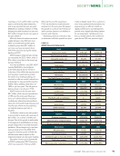
Feature Extraction and RNT Prediction
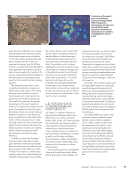
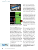
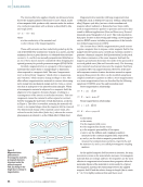
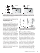
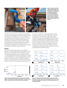
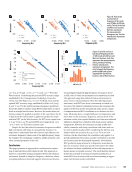
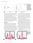
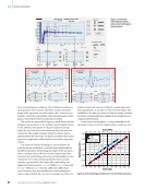
mRMR was performed on all 700 features to gauge the impor-
tance across different frequencies. The results are presented in
Figure 5a, where the importance is mapped against each indi-
vidual frequency. As mRMR is a mutual information quotient
that applies normalization by the total mutual information with
respect to other variables (i.e., frequencies), importance is a
value between 0 and 1 where the higher the value, the more
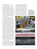
important it is. The locations of the most significant frequencies
are emphasized in Figure 5b. Here the FDD of all the training
and validation signals (35 +15) are plotted and the color map
indicates the normalized amplitude of each signal. The dash
lines signify the 30 most relevant features (i.e., frequencies). The
figure demonstrates that many extracted features coincide with
or are close to the peaks. In addition, the features align with very
low frequency information (i.e., 0–130 Hz).
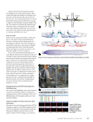
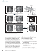
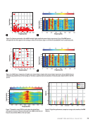
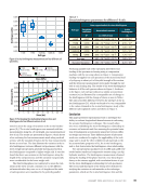
Similar to Figures 5a and 5b, Figures 6a and 6b present the
results obtained using NCA, which shares the same scope of
identifying the importance within a certain set of data but using
a different mathematical formulation with respect to mRMR.
NCA’s ordinate axis is represented by the weights associated with
each feature, enabling importances greater than one. Similar to
what was determined with mRMR, some of the most import-
ant frequencies lay around 50 Hz. This peak corresponds to the
so-called mode B, a translational mode in which the rail under-
goes a lateral deformation as a rigid body. This mode is strongly
affected by the boundary conditions and is highly governed by
the rail mass and the lateral resistance of the ties and fasteners.
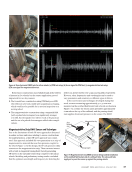
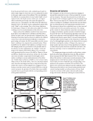
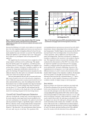
One noticeable difference between Figure 5b and Figure 6b is
that the relevant features determined with the NCA fall on the
peaks of the PSDs, whereas the relevant features determined with
mRMR reside around the valleys between consecutive peaks.
This is shown in Figure 7 for the peak around 350 Hz. Features
from both also tended to align on the 500 Hz peak, which is
linked to the so-called mode E, a temperature-dependent mode
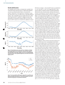
of vibration. These results are not surprising. The ground truth
RNT displayed in Figure 2 demonstrates that the boundary con-
ditions change daily with the ambient temperatures.
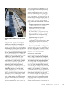
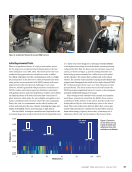
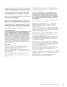
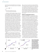
Finally, the following analyses were performed to quantify
the advantages about the use of a few frequencies with respect
to the full 0–700 Hz spectrum. Four feature sets were consid-
ered: one with all 700 frequencies, and one with the 100 most,
30 most, and 20 most relevant features, respectively. The latter
three were extracted with mRMR. The results are presented in
Figure 8, where the mean absolute error (MAE) between the
ME
|
RAILROADS
72
M A T E R I A L S E V A L U A T I O N • J A N U A R Y 2 0 2 4
2401 ME January.indd 72 12/20/23 8:01 AM
extraction, frequencies could then be constrained to those
associated with the RNT directly instead of the stress through
Equation 2. Removing the reliance on rail temperature addi-
tionally proves whether or not the impact of rail tempera-
ture can be modelled adequately using only PSD features
as opposed to explicitly providing it. It is noted here that for
feature extraction, models included only the lateral FDD as
input to demonstrate performance using a single direction.
The mRMR and the NCA algorithms were used to identify
the bandwidths most sensitive to stress and boundary condi-
tions. The first algorithm maximizes the relevance and mini-
mizes the redundancy of a set of data with respect to a certain
variable. This is done by using the maximum mutual informa-
tion quotient (MIQ):
(4) max
x ∈ Sc MIQx = max
x ∈ Sc
I(x, y) _
1
|S|
∑ z∈S I(x, z)
where
S is the number of features, and
I represents the mutual information.
In this study, S =700 to start because the PSD from which
the bandwidths are going to be identified spans from 0 to
700 Hz at 1 Hz frequency resolution. The mutual information I
measures how much the uncertainty of a random variable can
be reduced by knowing another variable. This is determined by
the following equation:
(5) I ( X, Z ) = ∑
i,j P(X = xi, Z = zj)log_______________ P(X = xi, Z = zj)
P(X = xi)P(Z = zj)
where
X and Z are random variables.
If the two variables are independent, I(X, Z) is equal to
zero. Therefore, to determine relevance and redundancy in the
PSD spectrums, the mRMR algorithm is used to maximize the
mutual information between a frequency and RNT whereas it
minimizes the mutual information between neighboring fre-
quencies. NCA is a nonparametric method that seeks to obtain
features that maximize the prediction accuracy of a regression
problem and acts as an alternative method to determining the
most prevalent features. This is accomplished by making use of
gradient descent to learn a distance metric by finding a linear
transformation of the input space. The distance metric takes
the following form:
(6) dw ( xi, xj ) = ∑
z=1
P wz 2 |xiz − xjz|
where
P represents the number of features (frequencies),
wz is feature weight, and
xiz and xjz are observations associated with said feature and a
random reference observation.
Weight vector w is optimized by approximating the reference
observation as a probability distribution allowing the residual
error between a prediction and target to be minimized with
optimization techniques like gradient descent. The distance
metric can then be utilized in the objective function where the
residual error between predicted and actual is weighted by the
probability of a sample belonging to the reference point. More
detailed implementations on both methods can be found in the
literature (Ding and Peng 2005 Yang et al. 2012).
Feature Extraction and RNT Prediction
mRMR was performed on all 700 features to gauge the impor-
tance across different frequencies. The results are presented in
Figure 5a, where the importance is mapped against each indi-
vidual frequency. As mRMR is a mutual information quotient
that applies normalization by the total mutual information with
respect to other variables (i.e., frequencies), importance is a
value between 0 and 1 where the higher the value, the more
important it is. The locations of the most significant frequencies
are emphasized in Figure 5b. Here the FDD of all the training
and validation signals (35 +15) are plotted and the color map
indicates the normalized amplitude of each signal. The dash
lines signify the 30 most relevant features (i.e., frequencies). The
figure demonstrates that many extracted features coincide with
or are close to the peaks. In addition, the features align with very
low frequency information (i.e., 0–130 Hz).
Similar to Figures 5a and 5b, Figures 6a and 6b present the
results obtained using NCA, which shares the same scope of
identifying the importance within a certain set of data but using
a different mathematical formulation with respect to mRMR.
NCA’s ordinate axis is represented by the weights associated with
each feature, enabling importances greater than one. Similar to
what was determined with mRMR, some of the most import-
ant frequencies lay around 50 Hz. This peak corresponds to the
so-called mode B, a translational mode in which the rail under-
goes a lateral deformation as a rigid body. This mode is strongly
affected by the boundary conditions and is highly governed by
the rail mass and the lateral resistance of the ties and fasteners.
One noticeable difference between Figure 5b and Figure 6b is
that the relevant features determined with the NCA fall on the
peaks of the PSDs, whereas the relevant features determined with
mRMR reside around the valleys between consecutive peaks.
This is shown in Figure 7 for the peak around 350 Hz. Features
from both also tended to align on the 500 Hz peak, which is
linked to the so-called mode E, a temperature-dependent mode
of vibration. These results are not surprising. The ground truth
RNT displayed in Figure 2 demonstrates that the boundary con-
ditions change daily with the ambient temperatures.
Finally, the following analyses were performed to quantify
the advantages about the use of a few frequencies with respect
to the full 0–700 Hz spectrum. Four feature sets were consid-
ered: one with all 700 frequencies, and one with the 100 most,
30 most, and 20 most relevant features, respectively. The latter
three were extracted with mRMR. The results are presented in
Figure 8, where the mean absolute error (MAE) between the
ME
|
RAILROADS
72
M A T E R I A L S E V A L U A T I O N • J A N U A R Y 2 0 2 4
2401 ME January.indd 72 12/20/23 8:01 AM


