
ground truth and the predicted RNT from the seven ML algo-
rithms is plotted for the four different feature sets. The MAE is
defined as:
(7) MAE = 1
n ∑
i=1
n |Yi − ˆi|
where
Yi is the value provided by the host, and
ˆ i is the value predicted by the algorithm.
Alongside the stratified sampling technique mentioned in
the Data Prepping section, fivefold cross validation was used
on every algorithm to gauge the performance of the models.
This also helps protect against overfitting by ensuring every
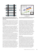
part of the dataset is accounted for in the training process. For
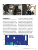
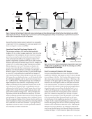
each algorithm, the number of bars in Figure 8 corresponds
to the number of varying parameters considered for the cor-
responding model, as shown in Table 1. For example, the LR
contains three bars per case compared to the six bars relative
to the SVM algorithm. Some results are not shown in Figure 8
because several linear models failed to learn from the 700
features. This was caused by either too many linear terms or
not enough observations compared to terms to perform the
regression task. Almost all the models apart from the GPR
show either an improvement or nearly no impact in perfor-
mance with the reduction in features to only the top 30 mRMR
frequencies demonstrating the significant redundancy of the
original PSDs. The GPR achieved the best performance among
any model tested. Although interpretability is difficult with
many of the tested algorithms, the GPR is beneficial given its
capability to provide a probabilistic prediction instead of a
fixed point prediction. This enables the use of prediction inter-
vals, which other models, such as traditional ANNs, are unable
to provide.
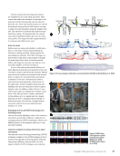
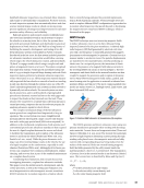
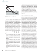
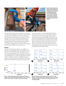
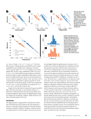
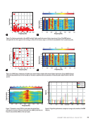
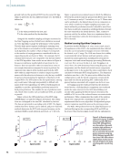
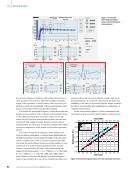
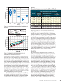
Figure 9 shows the GPR predictions of the RNT using
mRMR (Figure 9a) and NCA (Figure 9b) features. The estima-
tions are overlapped to the true RNT calculated by the host.
The data are presented in ascending order of RNT. The figures
confirm that fewer features can be utilized, and prove that both
methods determine the RNT with very good accuracy, as the
calculated MAE is nearly identical and about 0.2 °C for both.
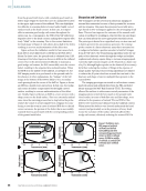
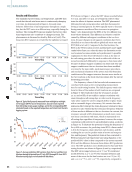
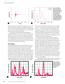
Figure 10 presents some isolated cases in which the difference
between the predicted and the ground truth RNT is more than
2.5 °C, between 34 and 36 °C as well as 30 to 32 °C. These cases
can be attributed to the limited data of 2021 in comparison to
2022, which contributes to higher sampling uncertainty con-
tained within the prediction intervals. It should be noted here
that these models also required no additional features beyond
the ones extracted in the lateral direction. Thus, contrary to
previous work by the authors, there is no requirement here to
have rail temperature unless the determination of stress from
RNT is desired.
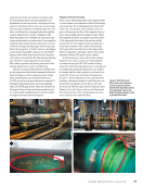
Machine Learning Algorithms Comparison
In previous studies (Belding et al. 2022, 2023a, 2023b, 2023c),
the application of the ANN to the experimental data collected
from the curved rail achieved margins of errors well within
the desired ±2.78 °C range. The ANN was chosen for its ability
to automatically extract features and learn patterns, as doc-
umented in many applications including but not limited to
computer vision and natural language processing (Krizhevsky
et al. 2012 He et al. 2015 Devlin et al. 2018 Thoppilan et al.
2022). There, the ANN determined stress using frequency, rail
temperature, and the lateral and vertical sensor components
as the input vector to the model. The stress could then be back
calculated to determine RNT using Equation 2. The frequency
resolution was also 0.1 Hz. The prior section differs from this
configuration as only the lateral component constituted the
input and was directly predicting RNT. Additionally, all fre-
quency features associated with a signal were fed in at once.
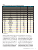
Leveraging upon the results presented in the aforemen-
tioned section, a full algorithmic comparison was conducted
under the same structure for the ANN from Belding et al.
(2023b) while applying the filtered features determined by
mRMR or NCA to see if the reduced feature sets retain similar
performance. Table 2 summarizes the results of the analyses,
which were computed by considering the same subset of
experimental data for every algorithm. All algorithm hyperpa-
rameter variations stayed the same as the previous section.
The Wide ANN performs best on the initial full feature set
(without filtering) as the corresponding MAE and MSE are
the lowest. This structure aligns closely with the optimization
ME
|
RAILROADS
300
Signal number
400
MAE: 0.229
MSE: 0.249
500 600 200 100
26
28
30
32
34
36
38
0
True responses
GPR predictions
300
Signal number
400
MAE:
MSE: 0.18338
500 600 200 100
26
28
30
32
34
36
0
True responses
GPR predictionsictionde
M 0.
E:
1
G prediction
00.2099.
MSE:
pr
Figure 9. (a) Gaussian process
regression using top 30 mRMR
features to predict RNT from
lateral FDD. Although there
are a few outliers, the model
maintains high confidence in
majority of predictions and
does so accurately: (b) Gaussian
process regression using top
30 NCA features to predict RNT
from lateral FDD. NCA achieves
slightly better results, but the
two sets of features are nearly
interchangeable in predicting
RNT.
74
M A T E R I A L S E V A L U A T I O N • J A N U A R Y 2 0 2 4
2401 ME January.indd 74 12/20/23 8:01 AM
RNT
(°C)
RNT
(°C)
rithms is plotted for the four different feature sets. The MAE is
defined as:
(7) MAE = 1
n ∑
i=1
n |Yi − ˆi|
where
Yi is the value provided by the host, and
ˆ i is the value predicted by the algorithm.
Alongside the stratified sampling technique mentioned in
the Data Prepping section, fivefold cross validation was used
on every algorithm to gauge the performance of the models.
This also helps protect against overfitting by ensuring every
part of the dataset is accounted for in the training process. For
each algorithm, the number of bars in Figure 8 corresponds
to the number of varying parameters considered for the cor-
responding model, as shown in Table 1. For example, the LR
contains three bars per case compared to the six bars relative
to the SVM algorithm. Some results are not shown in Figure 8
because several linear models failed to learn from the 700
features. This was caused by either too many linear terms or
not enough observations compared to terms to perform the
regression task. Almost all the models apart from the GPR
show either an improvement or nearly no impact in perfor-
mance with the reduction in features to only the top 30 mRMR
frequencies demonstrating the significant redundancy of the
original PSDs. The GPR achieved the best performance among
any model tested. Although interpretability is difficult with
many of the tested algorithms, the GPR is beneficial given its
capability to provide a probabilistic prediction instead of a
fixed point prediction. This enables the use of prediction inter-
vals, which other models, such as traditional ANNs, are unable
to provide.
Figure 9 shows the GPR predictions of the RNT using
mRMR (Figure 9a) and NCA (Figure 9b) features. The estima-
tions are overlapped to the true RNT calculated by the host.
The data are presented in ascending order of RNT. The figures
confirm that fewer features can be utilized, and prove that both
methods determine the RNT with very good accuracy, as the
calculated MAE is nearly identical and about 0.2 °C for both.
Figure 10 presents some isolated cases in which the difference
between the predicted and the ground truth RNT is more than
2.5 °C, between 34 and 36 °C as well as 30 to 32 °C. These cases
can be attributed to the limited data of 2021 in comparison to
2022, which contributes to higher sampling uncertainty con-
tained within the prediction intervals. It should be noted here
that these models also required no additional features beyond
the ones extracted in the lateral direction. Thus, contrary to
previous work by the authors, there is no requirement here to
have rail temperature unless the determination of stress from
RNT is desired.
Machine Learning Algorithms Comparison
In previous studies (Belding et al. 2022, 2023a, 2023b, 2023c),
the application of the ANN to the experimental data collected
from the curved rail achieved margins of errors well within
the desired ±2.78 °C range. The ANN was chosen for its ability
to automatically extract features and learn patterns, as doc-
umented in many applications including but not limited to
computer vision and natural language processing (Krizhevsky
et al. 2012 He et al. 2015 Devlin et al. 2018 Thoppilan et al.
2022). There, the ANN determined stress using frequency, rail
temperature, and the lateral and vertical sensor components
as the input vector to the model. The stress could then be back
calculated to determine RNT using Equation 2. The frequency
resolution was also 0.1 Hz. The prior section differs from this
configuration as only the lateral component constituted the
input and was directly predicting RNT. Additionally, all fre-
quency features associated with a signal were fed in at once.
Leveraging upon the results presented in the aforemen-
tioned section, a full algorithmic comparison was conducted
under the same structure for the ANN from Belding et al.
(2023b) while applying the filtered features determined by
mRMR or NCA to see if the reduced feature sets retain similar
performance. Table 2 summarizes the results of the analyses,
which were computed by considering the same subset of
experimental data for every algorithm. All algorithm hyperpa-
rameter variations stayed the same as the previous section.
The Wide ANN performs best on the initial full feature set
(without filtering) as the corresponding MAE and MSE are
the lowest. This structure aligns closely with the optimization
ME
|
RAILROADS
300
Signal number
400
MAE: 0.229
MSE: 0.249
500 600 200 100
26
28
30
32
34
36
38
0
True responses
GPR predictions
300
Signal number
400
MAE:
MSE: 0.18338
500 600 200 100
26
28
30
32
34
36
0
True responses
GPR predictionsictionde
M 0.
E:
1
G prediction
00.2099.
MSE:
pr
Figure 9. (a) Gaussian process
regression using top 30 mRMR
features to predict RNT from
lateral FDD. Although there
are a few outliers, the model
maintains high confidence in
majority of predictions and
does so accurately: (b) Gaussian
process regression using top
30 NCA features to predict RNT
from lateral FDD. NCA achieves
slightly better results, but the
two sets of features are nearly
interchangeable in predicting
RNT.
74
M A T E R I A L S E V A L U A T I O N • J A N U A R Y 2 0 2 4
2401 ME January.indd 74 12/20/23 8:01 AM
RNT
(°C)
RNT
(°C)


