Current methods to estimate RNT are based on strain
gages or the lift method. The first approach requires rail
cutting, prestressing, and re-welding (Wang et al. 2016). The lift
method requires unfastening 30 m of rail (Pandrol 2019). Pure
nondestructive testing (NDT) methods target the measurement
of the axial stress or the estimation of the RNT using physical
principles such as ultrasounds (Nucera et al. 2013 Nucera and
Lanza di Scalea 2014a, 2014b Lanza di Scalea and Nucera 2014
Szelaz˙ek ˛ 1992 Niu et al. 2023), digital image correlation (Knopf
et al. 2021), or acoustics (Bagheri et al. 2016 Nasrollahi and
Rizzo 2018, 2019), just to name a few. As the cross comparison
of these methodologies is beyond the scope of this paper, inter-
ested readers are referred to the review articles by Enshaeian
and Rizzo (2021) and Huang et al. (2023).
Over the past few years, the authors have developed an
NDT approach based on low-frequency vibrations, finite
element modeling, and machine learning (ML) (Enshaeian et
al. 2021 Belding et al. 2022, 2023a, 2023b, 2023c). The overar-
ching idea consists of triggering low-frequency (below 1 kHz)
vibrations of the rail of interest with a hammer and recording
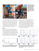
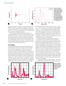
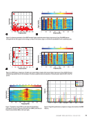
them with a few accelerometers. The power spectral densities
(PSD) of the vibrations are calculated from the time domain to
become part of the input vector of a ML algorithm developed
to associate the spectral densities with the longitudinal stress
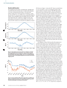
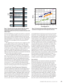
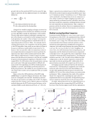
and then, using Equation 2, the RNT. The method was tested
in the field on a tangent track on wood crossties and a curved
track on concrete ties using an instrumented hammer and
wired and wireless accelerometers attached to the gage side of
the head. For both the tangent (Belding et al. 2023b) and the
curved rail (Belding et al. 2023c), it was found that an artificial
neural network (ANN) trained with experimental data was able
to predict the neutral temperature within the desired margin
of error of 2.78 °C. However, a few unanswered research ques-
tions remained, and the study presented in this paper answer
two of them, by analyzing the data collected from the curved
track on concrete ties. The first question pertained to the
performance of different ML algorithms to find the one that
outperforms the others in other words, the one that provides
the most accurate results in terms of neutral temperature pre-
dictions. The second question aimed to identify the number
of features, namely narrow bandwidths within the calculated
PSD, which are the most sensitive to the change of vibration
characteristics and neutral temperature. This second question
addresses the need to reduce the computational effort required
to train a “black box” algorithm with high dimensionality/
redundancy. This is because the extraction of exact features/
frequencies that are sensitive to stress is not trivial, especially
without the support of adequate modeling. To achieve the
first scope of the study, the following popular ML algorithms
were considered: linear regression (LR), decision trees, support
vector machine (SVM), ensembles, Gaussian process regres-
sion (GPR), and kernel approximation. These algorithms were
all trained and tested with the same set of experimental data.
To extract the relevant information for the PSDs, the minimum
redundancy–maximum relevance (mRMR) (Ding and Peng
2005) algorithm and the neighboring component analysis
(NCA) algorithm (Yang et al. 2012) were applied. mRMR seeks
to find the optimal set of features that maximize the relevance
and minimize the redundancy of a set of data to represent the
response variable effectively. Relevance is related to mutual
information between a feature and the output (RNT) and is
measured by using equations that will be presented later. NCA
is a nonparametric method that seeks to obtain features that
maximize the prediction accuracy of a regression problem and
acts as an alternative method to determining the most preva-
lent features.
This paper is organized as follows. The next section sum-
marizes the experimental setup and discusses the challenges
associated with the nondestructive estimation of the neutral
temperature. For the sake of completeness, this section also
describes the post-processing analysis of the experimental
vibrations. For more details, the reader is referred to Belding
et al. (2023a, 2023b). The Data Prepping section presents the
procedure to prep the input vector in support of the ML algo-
rithms. The Feature Extraction and RNT Prediction section
presents the results relative to the determination of the band-
width that should be considered to optimize the computational
efforts of the proposed vibration-based NDT. The section titled
ML Algorithms Comparison describes the results associated
with the determination of the algorithm that minimizes the
error between the predicted RNT and the ground RNT deter-
mined with a strain gage system. In addition, this section
includes an ablation study to measure the performance impact
of removing features from the models. Finally, the paper ends
with some concluding remarks.
Experiment
This section summarizes the experimental setup, discusses the
challenges associated with the nondestructive estimation of the
RNT, and describes the post-processing analysis of the experi-
mental vibrations.
Setup
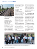
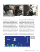
Two field tests were performed at the Transportation
Technology Center Inc. (TTCI) in Pueblo, Colorado, in May
2021 and May 2022. The center is a facility owned by the
Federal Railroad Administration, managed by MxV Rail (here-
inafter referred to as the host) at the time of the experiments.
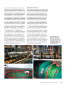
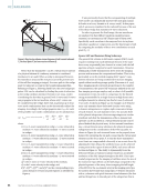
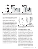
A tangent 136RE rail on wood crossties and a 5° curved 141RE
rail on concrete crossties were tested, and the data from the
latter were considered in this study. Vibrations on the rails
were induced with a hammer impacting the field side of the
railhead, in alternation above one tie and at the mid-span. The
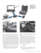
vibrations were recorded with a few accelerometers. In May
2021, two wired accelerometers were bonded to the rail. One
year later, two wireless accelerometers were added and all four
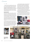
were attached to the rail using magnets instead of epoxy glue.
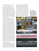
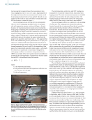
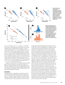
This latter setup is schematized in Figure 1. The performance
of the wireless accelerometers with respect to their wired coun-
terparts and the advantages of this modified setup are amply
ME
|
RAILROADS
68
M A T E R I A L S E V A L U A T I O N • J A N U A R Y 2 0 2 4
2401 ME January.indd 68 12/20/23 8:01 AM

discussed in Belding et al. (2023b, 2023c) and are not repeated
here. The other significant difference between 2021 and 2022 is
that in 2021 the number of samples collected (48 and 61) was
much smaller than one year later (415 and 531). The motivation
behind the difference is not related to the scope of this paper
but is related to a paradigmatic shift in the proposed NDT
approach.
The signals from the wired sensors were sampled at 10 kHz
using a signal conditioner and an oscilloscope. The signals
from the wireless gages were sampled at 4.096 kHz and sent
wirelessly directly to a laptop. Zero padding was applied to the
wireless data to achieve a frequency resolution equal to 0.1 Hz.
To gauge the temperature distribution within the rail, one
probe of a dual-type K/J input thermometer was placed on the
railhead, whereas the other probe was attached to the field side
of the web, which was mostly in the shade.
The host instrumented the rail with a conventional strain-
gage rosette bonded to the web of the rail and a temperature
sensor. While the temperature measurements by the host were
taken automatically every 5 min, the readings from the dual
thermometer were recorded manually every time the hammer
was used. Overall, the web readings from the K/J thermom-
eter are about 1–2 °C lower than the web readings from the
host. Both were located on the shady side of the rail, leading to
much less scattering compared to the head temperatures.
“Ground Truth” Neutral Temperature Estimations
The host calculated the “ground truth” neutral temperature of
the track using the strain-gage-based system installed on the
rail. Such calculations were provided to the authors by the host
and are presented in Figure 2. Specifically, Figure 2 shows the
RNT as a function of the corresponding rail host temperature
associated with the four days of testing on the curved track
(Figure 2). The data refer to the measurements taken between
9:00 a.m. and 2:00 p.m. of each day. The equations of the
corresponding linear regressions are presented as well, which
demonstrate a linear relationship between the RNT and the
steel temperature. Notably, Figure 2 demonstrates that the RNT
is proportional to the steel temperature even in the absence
of train operations, and it is different across days for the
same steel temperature. The latter is attributed to changes in
boundary conditions of the track due to the ambient tempera-
ture. This empirical evidence increases the challenge in the
nondestructive determination of the RNT. As a matter of fact,
the inherent variability associated with the ever-changing
boundary conditions makes the quantification of the axial
stress and thus RNT extremely challenging. In practice, the
longitudinal stress in Equation 2 is not only a function of the
difference between TR and TN but it is also a function of the
hourly (daily) changes of the boundary conditions. Both graphs
show that in May 2021 the RNT increased by less than 1 °C,
whereas in May 2022 the RNT increased almost 5 °C. This in
turn calls for a model capable of learning several boundary
conditions outside of simply changes in rail temperature.
Data Analysis
Figure 3a presents one of the time waveforms associated with
the lateral acceleration of the curved rail recorded on Day 1
by the sensor bonded at the mid-span when the excitation
occurred at the mid-span on the other side of the railhead. The
corresponding PSD along with the PSD of the vertical compo-
nent is shown in Figure 3b. The peaks around 150, 300, 470, and
680 Hz are flexural, torsional, or both modes. For example, the
mode at 680 Hz detected by the mid-span accelerometer when
the impacts were also at the mid-span is a flexural-torsional
mode with nodes at the crossties, thus “invisible” to the other
sensor. This mode is the so-called mode E, predicted numeri-
cally and extensively discussed in a previous paper (Belding et
al. 2022). The sensor, mounted on the portion of the railhead
above the crosstie, led to the detection of two additional
Wireless sensor–Tie
Wired sensor–Tie
Impact
location Wireless sensor–Mid
Wired sensor–Mid
Figure 1. Schematic of the test setup adopted in May 2022 showing
location of the two wireless and the two wired accelerometers
magnetically attached to the rail. The arrow indicates the location of the
hammer impact.
10
26
28
30
32
34
36
15 20 25
Rail temperature (°C)
30 35 40 45
D1
RNT
=0.18*T
R
+28.4 R2 =0.99
D2
RNT
=0.15*T
R
+26.9 R2 =0.98
D3
RNT
=0.10*T
R
+25.5 R2 =0.86
D4
RNT
=0.16*T
R
+27.6 R2 =0.95
Day 1 (2021)
Day 2 (2021)
Day 3 (2022)
Day 4 (2022)
Figure 2. Rail neutral temperature (RNT) estimated by the host using a
conventional strain-gage rosette for the inspected curved track.
J A N U A R Y 2 0 2 4 • M A T E R I A L S E V A L U A T I O N 69
2401 ME January.indd 69 12/20/23 8:01 AM
RNT
(°C)