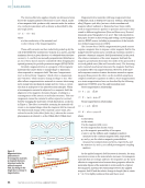
beyond the physical array element numbers) is a reasonable
compromise between imaging speed and image quality (reso-
lution and signal-to-noise ratio [SNR]).
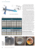
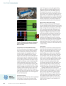
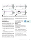
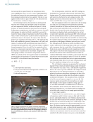
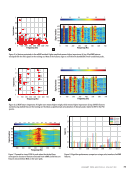
Quasi Real-Time Rail Flaw Image Display in 3D
The prototype includes a GUI that has been specifically
designed for the rail flaw imaging application. After the setup
configuration of the multiplexer, the user starts the scanning
process by moving the probe along the transverse direction
of the rail (perpendicularly to the imaging Y-Z plane). The
parallel computation capability of GPU in the host computer
achieves quasi real-time beamforming of the SAF images with
a frame rate of ~25 Hz using an eight-transmission modality
(Martin-Arguedas et al. 2012). The frame rate limit in the
system comes from the data transmission and conversion
hardware. The theoretical frame rate limit is much higher. As
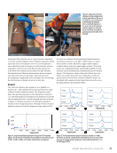
shown in Figure 6, the quasi real-time 3D point cloud display
is created by compounding the beamformed 2D images at
each transverse position tracked by the encoder. The raw 2D
SAF image slices are displayed using a –30 dB threshold while
the 3D display highlights only the pixels with intensity above
the –15 dB threshold. To distinguish image slices of different
signal strengths in the volumetric compounding, each 2D
image is normalized by the maximum intensity value in the
total collection of 3D pixels. Such a normalization process
calibrates the decibel levels of “noised” image slices to those
images with a strong reflection, suppressing any noise-only
pixels between different image slices. In the 3D display, the
algorithm performs this normalization adaptively by retain-
ing the maximum intensity value from the previous 2D image
and updating it if a larger maximum value is obtained. Notice
that the temporary display of the 3D point cloud is only for an
initial visualization of any strong reflections, including artifacts
that could affect the final size estimation. A post-processing
algorithm is needed to extract accurate quantitative informa-
tion regarding a possible internal flaw.
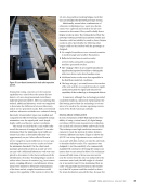
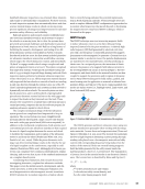
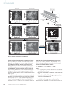
Post-Processing of Volumetric SAF Images
Post-processing algorithms have been developed to further
analyze the volumetric SAF images in order to extract the final
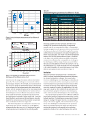
size and shape of the flaw. The flowchart illustrating the steps
taken in post-processing is shown in Figure 7. Referring to the
schematic on the upper right, the SAF image slices are beam-
formed in the vertical plane, while the final plane of interest
is the transverse plane. To prepare for image processing, the
point cloud is first resized to high resolution through bilinear
interpolation and converted from the decibel level (–40 to
0 dB) to an 8-bit grayscale, as shown in Figure 7a with two
sample slices both in the vertical plane and the transverse
plane. The volumetric image first goes through a coupled
dilation-erosion operation, where the intensity of each pixel
is first increased and then decreased based on the inten-
sity distribution of the neighboring pixels in 3D. As shown
in Figure 7b, the coupled morphology process blurs the void
between the grating lobes that are caused by Rayleigh diffrac-
tion limit of the beamformed ultrasonic waves. Following the
dilation and erosion operation, the volumetric image is flat-
tened to an identified noise level through filtering techniques,
as shown in Figure 7c. Each transverse plane slice is low-pass
Defect
Artifact
0
Length (mm)
Progress bar
Le ngth
(mm
)Slice (mm)
5
10
10
15
15
20
20
25
30
35
0
5
10
15
20
25
30
35
40 40
0
–5
–10
–15
–20
–25
–30 60 60 70 80 90 100
80
100
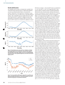
Indication of encoder position
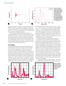
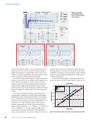
Figure 6. GUI runtime window displaying (a) compounded 3D point cloud
(–15 dB) and (b) raw 2D SAF image (–30 dB). The refreshing rate is 25 Hz
using the improved SAF technique.
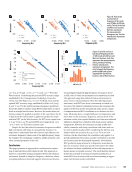
Focus
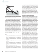
i =1
On-axis focus Off-axis focus
i =2
i =3 ROI
y
z
P (y, z)
ROI
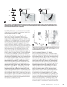
Figure 5. Subarray SAF technique for faster and more accurate images: (a) three defocused waves defined by the virtual elements are emitted
independently by subarrays. Beamforming in transmission is performed by applying time delays corresponding to a synthetic focus on point P
either at (b) on-axis positions or (c) off-axis positions.
J A N U A R Y 2 0 2 4 • M A T E R I A L S E V A L U A T I O N 55
2401 ME January.indd 55 12/20/23 8:01 AM
Depth
(mm)
Depth
(mm)

filtered and then subtracted from the original slice to flatten
the noise “phantoms.” From the sample slice in the vertical
plane, the smoothing process does not change the intensity
of the main lobe response. Since the noise floor is identi-
fied in each transverse plane, the volumetric intensity map
can finally be projected onto the transverse plane such that
the high intensity pixels are coherently added up, while the
lower intensity pixels remain at their intensity levels. Shown
in Figure 7d, after converting the grayscale image to decibel
levels, the example transverse defect is finally identified with a
high contrast.
At this point of the processing, it is necessary to isolate the
flaw from the background image. The critical step to highlight
the edge of the flaw is to apply a decibel level threshold and
convert the intensity map into a binary map. Typically, the
threshold is chosen as –15 dB for a ~30 dB dynamic range SAF
image, but the value should be adaptive to various circum-
stances such as defect orientation, reflectivity, SNR, and so
forth. In this paper a dynamic threshold level is determined
through the following empirical equation: ​ ​
(3)​ Threshold =a +b *cos(​θ​defect​​)​ ​ +c *noise​
where
{a, b, c} are empirical constants calibrated from ground truth
results from known flaws,
θdefect is the incident angle of the acoustic beams on the flaw,
and
noise is the decibel level of the background phantom deter-
mined in the flattening process.
To find the incident angle θdefect, the algorithm first
approximates the tilted angle φ of the flaw using the initial 3D
ME
|
RAILROADS
10
20
60 70 80 90 100
30
40
Length y (mm)
10
Vertical plane Transverse plane
Morphology
Filter
Binary
20
–20 –10 0
Horizontal plane
(x-y)
Defect
Artifact
Vertical plane
SAF image slices
(y-z)
Transverse plane
Final defect image
(x-z)
10 20
30
40
Transverse x (mm)
3D
10
20
60 70 80 90 100
30
40
Length y (mm)
10
20
–20 –10 0 10 20
30
40
Transverse x (mm)
10
20
–20 –10 0 10 20
30
40
Transverse x (mm)
10
20
–20 –10
Project to 2D
0 10 20
30
40
–10
0
–20
–30
Transverse x (mm)
3D
10
20
60 70 80 90 100
30
40
Length y (mm)
10
20
–20 –10 0 10 20
30
40
Transverse x (mm)
3D
x
z
y
Figure 7. Volumetric image post-processing flowchart.
56
M A T E R I A L S E V A L U A T I O N • J A N U A R Y 2 0 2 4
2401 ME January.indd 56 12/20/23 8:01 AM
Depth
z
(mm)
Depth
z
(mm)
Depth
z
(mm)
Depth
z
(mm)
Depth
z
(mm)
Depth
z
(mm)
Depth
z
(mm)
Depth
z
(mm)