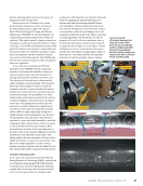
the transverse position of the probe when scanned on the
rail surface, with a resolution of 16 counts/mm. The encoder
allowed the system to create 3D images from the individual
2D scans. The array was coupled to the wedge using conven-
tional ultrasonic gel couplant. The couplant was also applied
at the wedge/rail interface to compensate for the impedance
mismatch. A graphical user interface (GUI) platform was devel-
oped on a standard commercial laptop with a GPU available
for parallel computation. All steps of the signal processing algo-
rithms were programmed and automated in the GUI platform,
which enabled flexible configuration and result analysis for the
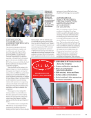
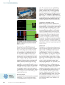
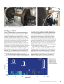
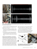
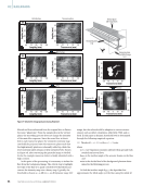
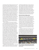
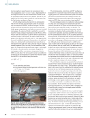
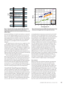
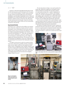
user’s convenience. As shown in Figure 3c, during testing the
user simply moves the probe on the surface of the rail section,
and 3D images of the scanned area are displayed in quasi real
time in the GUI.
Specific features of the image reconstruction algorithms
that were developed and implemented in the prototype are
discussed in detail in the following subsections.
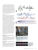
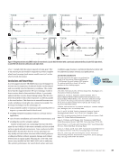
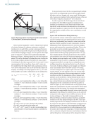
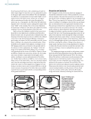
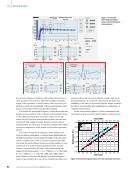
Time Backpropagation Beamforming with a Transducer
Wedge
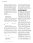
The time backpropagation algorithm (also known as
delay-and-sum or DAS algorithm) is widely used in SAF
imaging (Jensen et al. 2006). Dynamic focus is achieved both
in transmission and in reception by considering the ray path
connecting the transmitting transducer element, the focus
point, and the receiving transducer element. An image is
built by summing the backpropagated signals through all
transmitter-receiver pairs of the transducer array. Considering
transmitters i =1, 2,…, M and receivers j =1, 2,…, N, the DAS
beamformed SAF image is constructed as: ​ ​
(1)​ I(y, ​ z)​ =​ ∑
i=1​
M ​ ​ ∑
j=1​
N ​ ​ Ai​j​​​(​τ​ij,yz​​)​​​​
where
the time of flight (TOF) ​​ ​ ij,yz​​​ is the propagation time of the
ray path from the transmitter Ti(yi, zi) to the focus pixel
P(y, z) and back to the receiver Rj(yj, zj).
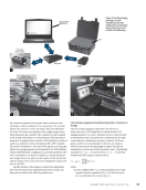
Ultrasonic array
(2.25 MHz, 64 elements)
Wedge
(55° shear wave)
Encoder
(16 counts/mm)
Case
Case
Battery
Multiplexer
Probe holder
(array+encoder)
Laptop computer
(MATLAB GUI)
Data
Data
Power
Laptop GUI
Handheld probe
Scan
direction
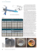
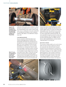
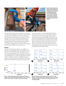
Figure 3. Portable imaging
prototype: (a) main
components (b) array-
wedge probe (c) prototype
during scanning of a rail
section in the laboratory.
J A N U A R Y 2 0 2 4 • M A T E R I A L S E V A L U A T I O N 53
2401 ME January.indd 53 12/20/23 8:01 AM

Notice that the transmitter i can be a virtual source instead
of a physical element if a subarray emission is considered
(Lockwood et al. 1998). When a wedge is interposed between
the transducer array and the test piece (as in the present case
of the rail flaw imaging prototype), the wave path in the wedge
must be taken into account in the beamforming algorithm.
Referring to Figure 4, following Snell’s law, the new backpropa-
gation TOF can be calculated by finding the point of refraction
at the wedge-medium interface (Sternini et al. 2019a, 2019b).
Considering the fact that, in general, both L-waves and S-waves
can propagate in the test medium, where only L-waves can
be considered in the wedge, there exist, in general, up to four
wave mode combinations that can be theoretically utilized for
imaging. Accordingly, the backpropagation time ​​ ​ ij,yz​​​ for each
of the possible wave mode combinations can be calculated as: ​ ​
(2)​ ​ ​ τ​ij,yz​​​​LLLL, LLSL, LSLL,LSSL​ =​ ​ di​L,y​(z​ 1)​​ _​
cw​​ ​ L ​
+​ ​ di​​L,y,S​(​2)​​ z _
cm,S​ ​ ​ L ​
+​ ​ dj​​Ly,S​(​3)​​ ,z _
cm,​S​ ​ L ​
+​ ​ dj​​Ly​(z​ ,4)​​ _
cw​​ ​ L ​ ​
where
LLLL is L-wave transmitted in wedge +L-wave refracted in
medium +L-wave reflected in medium +L-wave received
in wedge ,
LLSL is L-wave transmitted in wedge +L-wave refracted in
medium +S-wave reflected in medium +L-wave received
in wedge ,
LSLL is L-wave transmitted in wedge +S-wave refracted in
medium +L-wave reflected in medium +L-wave received
in wedge ,
LSSL is L-wave transmitted in wedge +S-wave refracted in
medium +S-wave reflected in medium +L-wave received
in wedge ,​ ​
c​m,​S​​ is the L-wave or S-wave velocity in the medium, ​ ​
c​w​​​ is the L-wave velocity in the wedge, and ​ ​
d​i,y​(z​ )​ ​ ​ ​​ ​ i,yz​ ​ (2)​ ​ ​ ​​ ​ j,yz​ ,​ (3)​ ​ ​ and ​​ ​ j,yz​ ​ ()​ ​ ​ are the corresponding propa-
gation distances of each ray path segment as identified in
Figure 4.
It was previously shown that the compounding of multiple
wave modes can dramatically increase the array gain (Lanza
di Scalea et al. 2017 Sternini et al. 2019a, 2019b). In this paper,
only S-waves are considered in the rail steel because of the use
of the shear wedge that maximizes S-wave refractions.
In order to generate the final image, the raw waveforms
are analyzed via their Hilbert transform (analytical repre-
sentation) as customary in SAF (Frazier and O’Brien 1998).
Specifically, each waveform is decomposed into its in-phase
and phase-quadrature components, and the final image is built
by computing the modulus of these two contributions at each
pixel P(y, z).
Sparse SAF and Emission Using Subarrays
The general SAF scheme in full matrix capture (FMC) mode
requires emitting from each individual element of the trans-
ducer array sequentially (one channel at a time) with the full
aperture acting in reception for each transmission. However,
utilizing all possible transmissions slows down the imaging
process and increases the computational burden. That is why,
particularly so in the medical imaging field, “sparse” trans-
mission schemes are being considered to increase imaging
speed without sacrificing image quality (Karaman et al. 1995).
Since imaging speed is inversely proportional to the number
of transmissions, the sparse SAF technique utilized in the rail
flaw imaging prototype employs only a subset of all possible
transmission events. In order to compensate for the limited
energy transmissible by a single element at high frame rates,
multiple elements (a subarray) are fired at once (Lockwood
et al. 1998). As shown in Figure 5a, for example, an 8-element
array only transmits three defocused circular waves using
3-element subapertures to replace eight consecutive firings
of each element. In each transmit event i, the acoustic field
of the phased subaperture elements superimposes a circular
wavefront such that the transmission of the 3-element sub-
aperture can be modeled as a virtual element (point source)
placed behind the physical array. In the transmit beamform-
ing, a virtual element array substitutes the physical transmit
subapertures in the consideration of the DAS ray paths. As
shown in Figure 5b, each transmit beam can be properly time
delayed by calculating the ray path connecting the virtual array
element and the focus point P, so that the three transmitted
wave fronts are compounded coherently at an on-axis focus. By
adjusting the time delays, the synthetic focus can be achieved
at any point in the region of interest (ROI), such as an off-axis
location in Figure 5c. The ability to dynamically focus the
defocused beams at various locations ensures an acceptable
resolution of the SAF images throughout the ROI. This is par-
ticularly important for the imaging of rail flaws since the size of
the transverse-type defects can be fairly large compared to the
physical aperture of the array, thus occupying the full height
of the ROI. For the 64-element array in the imaging prototype,
the authors have found that using eight, 17-element subarrays
with a 9-element-wide pitch between virtual elements (the first
and last firings have to discard part of the subaperture that is
ME
|
RAILROADS
Defect
Transducer array
Medium
Wedge
R
j
(y
j
,z
j
)
T
i
(y
i
,z
i
)
P(y, z)
θ
w
θ
m
d(1)
y
z
d(2)
d(4)
d(3)
Figure 4. Ray tracing scheme connecting one virtual transmit element
Ti, the focal point P, and one receiver element Rj.
54
M A T E R I A L S E V A L U A T I O N • J A N U A R Y 2 0 2 4
2401 ME January.indd 54 12/20/23 8:01 AM