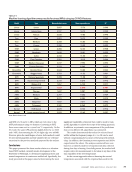
discussed in Belding et al. (2023b, 2023c) and are not repeated
here. The other significant difference between 2021 and 2022 is
that in 2021 the number of samples collected (48 and 61) was
much smaller than one year later (415 and 531). The motivation
behind the difference is not related to the scope of this paper
but is related to a paradigmatic shift in the proposed NDT
approach.
The signals from the wired sensors were sampled at 10 kHz
using a signal conditioner and an oscilloscope. The signals
from the wireless gages were sampled at 4.096 kHz and sent
wirelessly directly to a laptop. Zero padding was applied to the
wireless data to achieve a frequency resolution equal to 0.1 Hz.
To gauge the temperature distribution within the rail, one
probe of a dual-type K/J input thermometer was placed on the
railhead, whereas the other probe was attached to the field side
of the web, which was mostly in the shade.
The host instrumented the rail with a conventional strain-
gage rosette bonded to the web of the rail and a temperature
sensor. While the temperature measurements by the host were
taken automatically every 5 min, the readings from the dual
thermometer were recorded manually every time the hammer
was used. Overall, the web readings from the K/J thermom-
eter are about 1–2 °C lower than the web readings from the
host. Both were located on the shady side of the rail, leading to
much less scattering compared to the head temperatures.
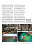
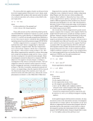
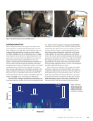
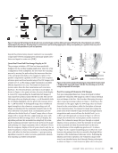
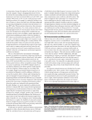
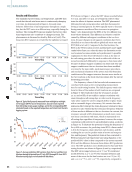
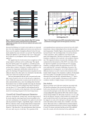
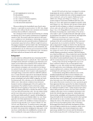
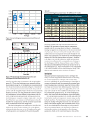
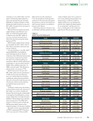
“Ground Truth” Neutral Temperature Estimations
The host calculated the “ground truth” neutral temperature of
the track using the strain-gage-based system installed on the
rail. Such calculations were provided to the authors by the host
and are presented in Figure 2. Specifically, Figure 2 shows the
RNT as a function of the corresponding rail host temperature
associated with the four days of testing on the curved track
(Figure 2). The data refer to the measurements taken between
9:00 a.m. and 2:00 p.m. of each day. The equations of the
corresponding linear regressions are presented as well, which
demonstrate a linear relationship between the RNT and the
steel temperature. Notably, Figure 2 demonstrates that the RNT
is proportional to the steel temperature even in the absence
of train operations, and it is different across days for the
same steel temperature. The latter is attributed to changes in
boundary conditions of the track due to the ambient tempera-
ture. This empirical evidence increases the challenge in the
nondestructive determination of the RNT. As a matter of fact,
the inherent variability associated with the ever-changing
boundary conditions makes the quantification of the axial
stress and thus RNT extremely challenging. In practice, the
longitudinal stress in Equation 2 is not only a function of the
difference between TR and TN but it is also a function of the
hourly (daily) changes of the boundary conditions. Both graphs
show that in May 2021 the RNT increased by less than 1 °C,
whereas in May 2022 the RNT increased almost 5 °C. This in
turn calls for a model capable of learning several boundary
conditions outside of simply changes in rail temperature.
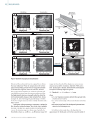
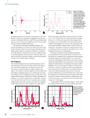
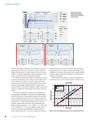
Data Analysis
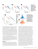
Figure 3a presents one of the time waveforms associated with
the lateral acceleration of the curved rail recorded on Day 1
by the sensor bonded at the mid-span when the excitation
occurred at the mid-span on the other side of the railhead. The
corresponding PSD along with the PSD of the vertical compo-
nent is shown in Figure 3b. The peaks around 150, 300, 470, and
680 Hz are flexural, torsional, or both modes. For example, the
mode at 680 Hz detected by the mid-span accelerometer when
the impacts were also at the mid-span is a flexural-torsional
mode with nodes at the crossties, thus “invisible” to the other
sensor. This mode is the so-called mode E, predicted numeri-
cally and extensively discussed in a previous paper (Belding et
al. 2022). The sensor, mounted on the portion of the railhead
above the crosstie, led to the detection of two additional
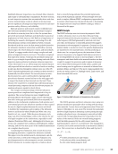
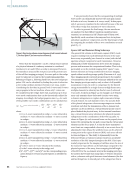
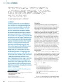
Wireless sensor–Tie
Wired sensor–Tie
Impact
location Wireless sensor–Mid
Wired sensor–Mid
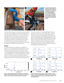
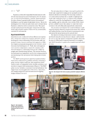
Figure 1. Schematic of the test setup adopted in May 2022 showing
location of the two wireless and the two wired accelerometers
magnetically attached to the rail. The arrow indicates the location of the
hammer impact.
10
26
28
30
32
34
36
15 20 25
Rail temperature (°C)
30 35 40 45
D1
RNT
=0.18*T
R
+28.4 R2 =0.99
D2
RNT
=0.15*T
R
+26.9 R2 =0.98
D3
RNT
=0.10*T
R
+25.5 R2 =0.86
D4
RNT
=0.16*T
R
+27.6 R2 =0.95
Day 1 (2021)
Day 2 (2021)
Day 3 (2022)
Day 4 (2022)
Figure 2. Rail neutral temperature (RNT) estimated by the host using a
conventional strain-gage rosette for the inspected curved track.
J A N U A R Y 2 0 2 4 • M A T E R I A L S E V A L U A T I O N 69
2401 ME January.indd 69 12/20/23 8:01 AM
RNT
(°C)

frequencies around 370 and 530 Hz, not shown here. Due to the
hammer being driven manually, the amplitudes of the spectra
were not constant and, therefore, each PSD was normalized with
respect to its own maximum amplitude to remove any potential
bias caused by the strength of the impact.
Not shown here but amply discussed in Belding et al.
(2023b) and Belding et al. (2023c), the PSD between the wired
and the wireless sensors were quite similar, with the latter pro-
viding a better signal-to-noise ratio. In addition, the frequen-
cies of the peaks on a given day were not necessarily the same
on the following day, or from one year to the next. This is con-
sistent with what is discussed in Figure 2 and is likely related to
a change in the rail’s boundary conditions.
Data Prepping
The instrumented hammer was operated manually, as previ-
ously mentioned. Due to the stochastic nature of the impact
force, min-max normalization was chosen to remove any
inherent bias associated with the variable strength of the
impact. It is noted here that the signals were not normalized by
the hammer’s maximum value, as one of the long-term objec-
tives of the project is to simplify the setup. As such, the use of a
regular hammer without the need for a signal conditioner and
a digitizer to record the impulsive force is preferable. Datasets
were clustered with respect to the tie material, and a stratified
sampling technique was used across each day. This sampling
scheme split the data into train/validation/test splits, which
kept the percentage taken from each day the same. The split
35-15-50 was considered in the study presented in this paper,
where (35 +15) is the percentage of the data samples used
for training 15 is the percentage of the training data used to
validate the learning process and 50 is the percentage of the
never-presented-before samples used to predict the neutral
temperature. This split was chosen as it represents the worst-
case split out of previous studies by the authors due to it con-
taining the least amount of training data.
The lateral component of the vibration measured by
the accelerometers on the rail above the tie and above the
mid-span were combined into a single signal using frequency
domain decomposition (FDD) (Brincker et al. 2001). FDD
consists of computing the PSD matrix for all sensor locations
and performing singular value decomposition of the matrix to
obtain the singular values. Leveraging upon previous studies
(Belding et al. 2023), the frequency range 0–700 Hz and res-
olution of 0.1 Hz were considered, and the head temperature
measured with the K/J thermometer was considered for two
reasons. The head temperature may be closer to the tem-
perature distribution across the whole rail cross section than
the temperature recorded from the web located in the shade.
Second, the number and the timeline of samples taken with
the K/J thermometer were identical to the acceleration data,
easing the overall analysis.
A representative FDD is provided in Figure 4, which shows
the combined PSD via FDD associated with the wired and
ME
|
RAILROADS
0
0
–0.5
–1
0.5
1
–0.05 0.05
Time (s)
0.1 0.15 0.2 0
0
0.2
0.4
0.6
0.8
1
200 400 600 800 1000
Frequency (Hz)
Lateral
Vertical
Figure 3. (a) typical
time series associated
with the lateral impact
applied at the mid-span
and recorded by the
accelerometer at the
mid-span on Day 1
(concrete) in May 2021
(b) corresponding power
spectral density (PSD)
overlapped to the PSD of
the vertical direction.
0
0.2
0.4
0.6
0.8
1
0
0
0.2
0.4
0.6
0.8
1
200 100 400 300 600 500 700
Frequency (Hz)
0 200 100 400 300 600 500 700
Frequency (Hz)
Figure 4. Example
of pooled spectral
information via FDD:
(a) lateral direction
and (b) vertical
direction.
70
M A T E R I A L S E V A L U A T I O N • J A N U A R Y 2 0 2 4
2401 ME January.indd 70 12/20/23 8:01 AM
Amplitude
(V)
PSD
amplitude
×
10–6
Normalized
amplitude
Normalized
amplitude