
wireless sensor. The FDD encompassed the only input to the
models for feature extraction so we could remove any reliance
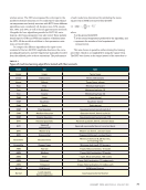
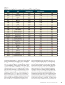
on temperature and strictly associate with RNT. Seven different
algorithms were considered: LR, decision trees, SVM, ensem-
bles, GPR, and ANN, as well as kernel approximation methods.
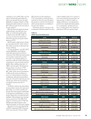
Alongside the base algorithms provided in MATLAB, varia-
tions in a few base parameters were also tested. These include
kernel type for GPRs and SVMs and number of hidden layers
for ANN. All the models in addition to their parameter varia-
tions are listed Table 1.
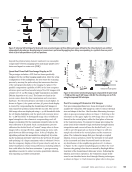
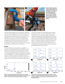
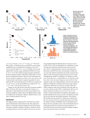
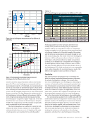
To compare the different algorithms, the input vector
consisted of the two full FDD amplitude directions, the corre-
sponding frequencies, and the temperature manually recorded
from the railhead probe at those excitations. The performance
of each model was determined by calculating the mean-
squared error (MSE) associated with the RNT:
(3) MSE = 1
n ∑
i=1
n
( Yi − ˆ i )
2
where
Yi is the ground truth RNT,
ˆ i is the neutral temperature predicted by the algorithm, and
n represents the number of total experimental
measurements.
This was chosen to penalize outliers during the training
procedure, which is accomplished by using the square term.
The RNT was chosen as the target instead of the stress due to
T A B L E 1
Types of machine learning algorithms tested with their variants
Model Type Note
Linear Linear Terms linear
Linear Interactions Terms interactions
Linear Robust Terms linear, robust
Tree Fine Minimum leaf size 4
Tree Medium Minimum leaf size 12
Tree Coarse Minimum leaf size 36
SVM Linear Linear kernel
SVM Quadratic Quadratic kernel
SVM Cubic Cubic kernel
SVM Fine Gaussian Gaussian kernel, kernel scale 6.6
SVM Medium Gaussian Gaussian kernel, kernel scale 26
SVM Coarse Gaussian Gaussian kernel, kernel scale 110
GPR Rational quadratic Rational quadratic kernel, constant basis
GPR Squared
exponential Squared exponential kernel, constant basis
GPR Matern 5/2 Matern 5/2 kernel, constant basis
GPR Exponential Exponential kernel, constant basis
Ensemble Boosted trees Minimum leaf size 8, 30 learners,
0.1 learning rate
Ensemble Bagged trees Minimum leaf size 8, 30 learners
ANN Narrow 1 layer, ReLU activation, 10 nodes
ANN Medium 1 layer, ReLU activation, 25 nodes
ANN Wide 1 layer, ReLU activation, 100 nodes
ANN Bilayered 2 layer, ReLU activation, 10 nodes each
ANN Trilayered 3 layer, ReLU activation, 10 nodes each
Kernel SVM kernel SVM kernel learner
Kernel Least-squares
kernel regression Least-squares kernel learner
J A N U A R Y 2 0 2 4 • M A T E R I A L S E V A L U A T I O N 71
2401 ME January.indd 71 12/20/23 8:01 AM
models for feature extraction so we could remove any reliance
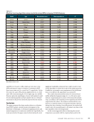
on temperature and strictly associate with RNT. Seven different
algorithms were considered: LR, decision trees, SVM, ensem-
bles, GPR, and ANN, as well as kernel approximation methods.
Alongside the base algorithms provided in MATLAB, varia-
tions in a few base parameters were also tested. These include
kernel type for GPRs and SVMs and number of hidden layers
for ANN. All the models in addition to their parameter varia-
tions are listed Table 1.
To compare the different algorithms, the input vector
consisted of the two full FDD amplitude directions, the corre-
sponding frequencies, and the temperature manually recorded
from the railhead probe at those excitations. The performance
of each model was determined by calculating the mean-
squared error (MSE) associated with the RNT:
(3) MSE = 1
n ∑
i=1
n
( Yi − ˆ i )
2
where
Yi is the ground truth RNT,
ˆ i is the neutral temperature predicted by the algorithm, and
n represents the number of total experimental
measurements.
This was chosen to penalize outliers during the training
procedure, which is accomplished by using the square term.
The RNT was chosen as the target instead of the stress due to
T A B L E 1
Types of machine learning algorithms tested with their variants
Model Type Note
Linear Linear Terms linear
Linear Interactions Terms interactions
Linear Robust Terms linear, robust
Tree Fine Minimum leaf size 4
Tree Medium Minimum leaf size 12
Tree Coarse Minimum leaf size 36
SVM Linear Linear kernel
SVM Quadratic Quadratic kernel
SVM Cubic Cubic kernel
SVM Fine Gaussian Gaussian kernel, kernel scale 6.6
SVM Medium Gaussian Gaussian kernel, kernel scale 26
SVM Coarse Gaussian Gaussian kernel, kernel scale 110
GPR Rational quadratic Rational quadratic kernel, constant basis
GPR Squared
exponential Squared exponential kernel, constant basis
GPR Matern 5/2 Matern 5/2 kernel, constant basis
GPR Exponential Exponential kernel, constant basis
Ensemble Boosted trees Minimum leaf size 8, 30 learners,
0.1 learning rate
Ensemble Bagged trees Minimum leaf size 8, 30 learners
ANN Narrow 1 layer, ReLU activation, 10 nodes
ANN Medium 1 layer, ReLU activation, 25 nodes
ANN Wide 1 layer, ReLU activation, 100 nodes
ANN Bilayered 2 layer, ReLU activation, 10 nodes each
ANN Trilayered 3 layer, ReLU activation, 10 nodes each
Kernel SVM kernel SVM kernel learner
Kernel Least-squares
kernel regression Least-squares kernel learner
J A N U A R Y 2 0 2 4 • M A T E R I A L S E V A L U A T I O N 71
2401 ME January.indd 71 12/20/23 8:01 AM


