
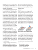
results achieved in Belding et al. (2023a, 2023c) where sufficient
function approximation could be done using a single hidden
layer. When converting stress to RNT with Equation 2 for the
wide ANN results, the respective MAE and MSE are 1.084 and
1.74 °C, well within the required 2.78 °C design criteria. Some
algorithms such as SVM and GPR did not converge and failed.
This was attributed to the O(n3) complexities that SVM and
GPRs have when the number of observations grow. As each
frequency is treated as a separate observation to allow for a
comparative study to Belding et al. (2023b, 2023c), the com-
plexities grow to (7000 ∗ 517)3 where 7000 is the number of
frequencies in a PSD here (0.1 Hz resolution) and 517 is the
number of samples in training and validation. It is also noted
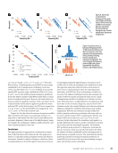
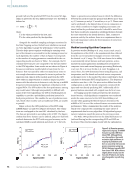
that even though the neural networks performed the best,
there was still a lack in performance in comparison to the
network trained in prior work that had an MAE of 0.50 °C,
which can be attributed to the absence of hyperparameter
search steps taken here. Tree-based methods performed the
next best, which included the ensembles as well as regular
decision trees close behind. They did, however, suffer more
when it came to capturing relative outliers as the MSE was
higher than that of the neural network with 8.86 and 14.63
compared to the ANN’s 6.69 MSE. The linear SVM was the
only SVM to converge of the available six and performed the
poorest from not only a stress prediction standpoint but a
computational one as well. Due to the computational cost of
predictions from the SVM compared to all other algorithms
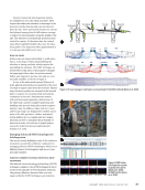
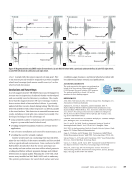
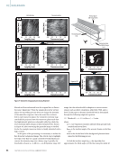
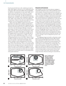
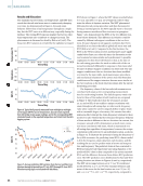
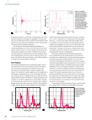
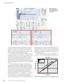
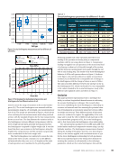
using all features, Figure 10 presents a histogram of errors for
the best model and second to worst (Fine Tree). Both demon-
strate from an average residual error desired performance to
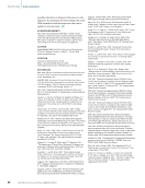
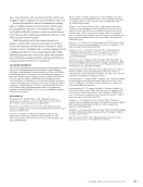
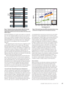
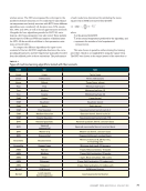
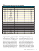
T A B L E 2
Machine learning algorithm sweep results for stress (MPa) using all features
Model Type Mean absolute error Mean-squared error R2
Linear Linear 3.159 15.12 0.949
Linear Interactions 3.111 14.64 0.951
Linear Robust 3.084 15.40 0.948
Tree Fine 2.341 15.47 0.948
Tree Medium 2.330 15.32 0.948
Tree Coarse 2.329 15.20 0.949
SVM Linear 5.006 36.06 0.878
SVM Quadratic NaN NaN NaN
SVM Cubic NaN NaN NaN
SVM Fine Gaussian NaN NaN NaN
SVM Medium Gaussian NaN NaN NaN
SVM Coarse Gaussian NaN NaN NaN
Ensemble Boosted trees 2.610 10.63 0.964
Ensemble Bagged trees 1.880 8.857 0.970
GPR Rational quadratic NaN NaN NaN
GPR Squared exponential NaN NaN NaN
GPR Matern 5/2 NaN NaN NaN
GPR Exponential NaN NaN NaN
ANN Narrow 2.136 8.438 0.971
ANN Medium 2.051 7.833 0.974
ANN Wide 1.843 6.700 0.977
ANN Bilayered 2.019 7.886 0.973
ANN Trilayered 2.021 7.945 0.973
Kernel SVM kernel 2.941 12.23 0.959
Kernel Least-squares kernel 2.884 12.40 0.958
Note: Best is shown in red
J A N U A R Y 2 0 2 4 • M A T E R I A L S E V A L U A T I O N 75
2401 ME January.indd 75 12/20/23 8:01 AM
function approximation could be done using a single hidden
layer. When converting stress to RNT with Equation 2 for the
wide ANN results, the respective MAE and MSE are 1.084 and
1.74 °C, well within the required 2.78 °C design criteria. Some
algorithms such as SVM and GPR did not converge and failed.
This was attributed to the O(n3) complexities that SVM and
GPRs have when the number of observations grow. As each
frequency is treated as a separate observation to allow for a
comparative study to Belding et al. (2023b, 2023c), the com-
plexities grow to (7000 ∗ 517)3 where 7000 is the number of
frequencies in a PSD here (0.1 Hz resolution) and 517 is the
number of samples in training and validation. It is also noted
that even though the neural networks performed the best,
there was still a lack in performance in comparison to the
network trained in prior work that had an MAE of 0.50 °C,
which can be attributed to the absence of hyperparameter
search steps taken here. Tree-based methods performed the
next best, which included the ensembles as well as regular
decision trees close behind. They did, however, suffer more
when it came to capturing relative outliers as the MSE was
higher than that of the neural network with 8.86 and 14.63
compared to the ANN’s 6.69 MSE. The linear SVM was the
only SVM to converge of the available six and performed the
poorest from not only a stress prediction standpoint but a
computational one as well. Due to the computational cost of
predictions from the SVM compared to all other algorithms
using all features, Figure 10 presents a histogram of errors for
the best model and second to worst (Fine Tree). Both demon-
strate from an average residual error desired performance to
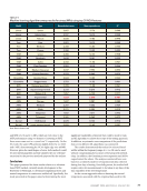
T A B L E 2
Machine learning algorithm sweep results for stress (MPa) using all features
Model Type Mean absolute error Mean-squared error R2
Linear Linear 3.159 15.12 0.949
Linear Interactions 3.111 14.64 0.951
Linear Robust 3.084 15.40 0.948
Tree Fine 2.341 15.47 0.948
Tree Medium 2.330 15.32 0.948
Tree Coarse 2.329 15.20 0.949
SVM Linear 5.006 36.06 0.878
SVM Quadratic NaN NaN NaN
SVM Cubic NaN NaN NaN
SVM Fine Gaussian NaN NaN NaN
SVM Medium Gaussian NaN NaN NaN
SVM Coarse Gaussian NaN NaN NaN
Ensemble Boosted trees 2.610 10.63 0.964
Ensemble Bagged trees 1.880 8.857 0.970
GPR Rational quadratic NaN NaN NaN
GPR Squared exponential NaN NaN NaN
GPR Matern 5/2 NaN NaN NaN
GPR Exponential NaN NaN NaN
ANN Narrow 2.136 8.438 0.971
ANN Medium 2.051 7.833 0.974
ANN Wide 1.843 6.700 0.977
ANN Bilayered 2.019 7.886 0.973
ANN Trilayered 2.021 7.945 0.973
Kernel SVM kernel 2.941 12.23 0.959
Kernel Least-squares kernel 2.884 12.40 0.958
Note: Best is shown in red
J A N U A R Y 2 0 2 4 • M A T E R I A L S E V A L U A T I O N 75
2401 ME January.indd 75 12/20/23 8:01 AM


