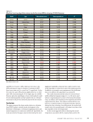
testing day. Each vibration test at a given location comprised
10 or more repeated impulse-driven vibration responses, which
represents one set of responses. Five to 13 sets of responses
were collected at each test location on each test day, and con-
sequently a total of 73 sets at the East location and 65 sets
at the West were collected across all the test days. Because
this impulse-based vibration measurement does not require
any mounted sensors or rail surface and track structure
pre-preparation, application of the technique does not damage
the rail structure or disrupt rail service in any way.
Analysis
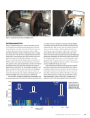
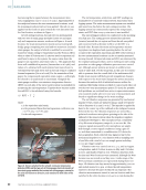
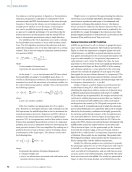
The collected vibration time signals are zero-padded to a
duration of 1 s and transformed into spectral responses using
a discrete Fourier transform routine. The frequency resolu-
tion of the spectral responses is 1 Hz. The spectra of each set
(~10 repeated signals) are averaged across frequency to provide
one averaged spectrum. A typical averaged spectrum is shown
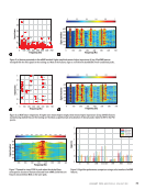
in Figure 4. Vibration resonances are identified as peaks or
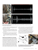
maxima in the averaged spectrum. Although several resonance
peaks are observed in the low frequency range under 20 kHz,
we focus our attention on four prominent higher frequency
resonances around 31, 37, 39, and 76 kHz because we expect
these modes to not be affected by support and boundary
condition effects such as tie span length variation. These four
modes are consistently present and visually trackable at both
locations across all testing days, as illustrated in more detail in
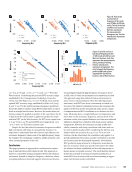
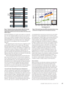
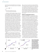
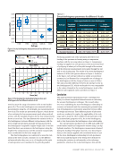
Figure 5. The frequency values at the peak of these four reso-
nances are tracked across the nine testing days, and the fre-
quency values of each of the monitored vibration modes are
correlated with measured strain values that occur at the corre-
sponding vibration measurement times.
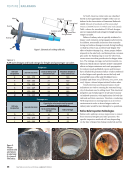
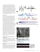
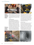
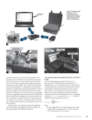
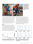
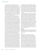
Condenser microphone
Steel impactor
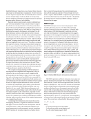
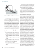
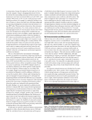
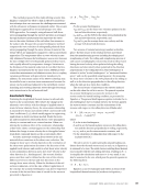
Figure 3. Illustration of (a) the
vibration testing configuration
and (b) application of the test at
the field site. The rail vibration
is initiated by the impulse
from a steel ball impactor at
the center-top of the railhead,
and the response is collected
by the condenser microphone
pointing toward the side of the
railhead.
20 000 0
0.0000
0.0002
0.0004
0.0006
40 000 60 000
Frequency (Hz)
80 000 100 000 120 000
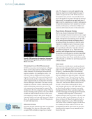
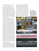
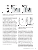
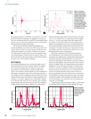
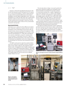
Figure 4. A typical amplitude spectrum averaged over 10 repeated
signals. The red arrows indicate the four prominent resonances around
31 kHz, 37 kHz, 39 kHz, and 76 kHz, which will be investigated.
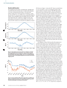
5 August
15 August
29 August
5 August
15 August
29 August
5 Augustu
15 Augustu
29 Augustu
5
15
29
30 800 31 000 31 200 31 400 31 600
Frequency (Hz)
36 800 37 000 37 200 37 400
Frequency (Hz)
39 000 39 200 39 400 39 600 39 800
Frequency (Hz)
76 200 76 400 76 600 76 800
Frequency (Hz)
77 000
s
s
s
AAugust
AAugust
AAugust
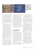
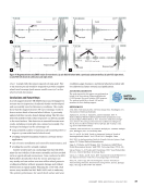
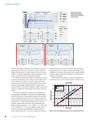
Figure 5. The four prominent spectral resonances around (a) 31 kHz
(b) 39 kHz (c) 37 kHz and (d) 76 kHz (indicated by arrows in cases of the
presence of multiple peaks nearby) are consistently identified on 5, 15,
and 29 August 2019.
J A N U A R Y 2 0 2 4 • M A T E R I A L S E V A L U A T I O N 63
2401 ME January.indd 63 12/20/23 8:01 AM
Amplitude

Results and Discussion
The regularly reported strain, rail temperature, and RNT data
reveal that the rail axial stress state is continuously changing
over time. As demonstrated in Figure 6, the axial strain
behavior follows that of rail temperature throughout a single
day, but the RNT varies in a different way, especially during the
daytime. The varying RNT response implies that factors other
than temperature also contribute to changes in strain. The
phenomenon is discussed in detail by Kish et al. (1987). The
long-term RNT variation is revealed by the nighttime averaged
RNT shown in Figure 7, where the RNT values recorded before
6:00 a.m. and after 7:00 p.m. are averaged in order to elim-
inate the effects of daytime variation. The RNT plummeted
following the rail-cutting procedure and then fluctuates fol-
lowing a seasonal pattern: the RNT typically starts to decrease
during summer months and then increases in springtime.
Figure 7 also demonstrates the RNTs at the two different loca-
tions behave distinctly. This difference in behavior could be
caused by different rail support conditions at the two loca-
tions, because changes in rail support conditions have been
identified as one factor that affects global rail stress state and
RNT (Kish et al. 1987). Compared to the East location, the
RNT on the West location is lower and fluctuates more signifi-
cantly before June 2020 after this time, the fluctuation at the
two locations becomes similar and synchronized. A possible
explanation for this observed behavior is that at the time of
the rail-cutting procedure the track on either side of the cut
moved (contracted) differently in response to that stress relief
because of distinct support conditions on either side. The rail
support conditions at the two locations have been modified
over time by the train traffic, track maintenance procedures,
and mechanical relaxation of the system such that boundary
conditions and the support structure become more similar at
the two locations as the track structure relaxes after the rail cut
destressing procedure.
The frequency values of the four selected resonances are
correlated with strain at the corresponding measurement
time for each testing location. The daily frequency-strain rela-
tions for three of the modes at both locations are compared
in Figure 8. The results show that the resonances around
37, 39, and 76 kHz do not exhibit a unique correlation with
strain throughout all testing days in other words, frequency
value alone cannot be used to uniquely define in-place strain
with a reasonable degree of accuracy. We surmise that other
unknown effects disrupt the strain-frequency relation for these
modes. It is also evident that the resonance frequency behavior
of these modes is different at the two locations. In contrast, the
resonance around 31 kHz demonstrates a much more consis-
tent linear correlation with strain, which is maintained over
all testing days regardless of temperature however, the unique
correlation is still restricted to an individual location, as shown
in Figure 9a. To illustrate the potential of using the frequency of
the 31 kHz resonance for predicting strain/RNT, a linear model
is fit to the frequency-strain data from each location, and the
resulting fits are used to predict strain at known rail tempera-
ture and frequency. The predicted strain is then converted to
RNT, knowing the rail temperature and using Equation 2 the
predicted RNT value is then compared to the system-reported
RNT, and the difference between them defines RNT prediction
error. The RNT prediction error distributions for East and West
testing locations are shown in Figures 9b and 9c, respectively.
The RNT errors range between ±3.33 °C (±6 °F) overall and
mostly between ±1.11 °C (±2 °F). The standard deviation and
mean of the errors for the East location are ±1.16 °C (±2.1 °F)
and –1.61 × 10–9 °C (–2.87 × 10–9 °F), respectively, compared to
ME
|
RAILROADS
Time of day
Time of day
00:00 03:00 06:00 09:00 12:00 15:00 18:00 21:00 00:00
Time of day
00:00
100
100
80
60
92
91
90
0
–100
–200
03:00 06:00 09:00 12:00 15:00 18:00 21:00 00:00
00:00 03:00 06:00 09:00 12:00 15:00 18:00 21:00 00:00
Figure 6. Typical daily records measured from midnight to midnight
on 15 August 2019 of (a) rail temperature (b) axial strain reported
from full-bridge strain gauge readings and (c) the corresponding RNT
calculated based on the reported temperature and strain from the data
logging system.
Date
2019- 09 2019- 11 2020- 01 2020- 03 2020- 05 2020- 07 2020- 09 2020- 11 2021- 01 2021- 03 2021- 05
65
70
75
80
85
90
East
West
Test days
Figure 7. Average nighttime RNT variation from the East and West test
locations during the period from 31 July 2019 through 20 June 2021.
Vibration testing days are indicated with black dots.
64
M A T E R I A L S E V A L U A T I O N • J A N U A R Y 2 0 2 4
2401 ME January.indd 64 12/20/23 8:01 AM
RNT
(°F)
Microstrain
T
(°F)
RNT
(°F)