Considering an excitation signal with a time width of N c =
5 cycles and a center frequency f k selected from an N w -point
sweep-frequency set W sweep ={f 1 ,⋯ ,f k ⋯,fNw}, the probing
signal s t (k) can be written (Ren et al. 2023, 2025a, 2025b) as:
(2) s t (k) =exp
[
− t ⊙ t _
2 (N c _
2 √ _
2ln2 )f k ]
⊙ 0.5
{
1 − cos
[
2πt
(
N c
f k )]}
⊙ sin(2πfkt)
↓ ↓ ↓
Gaussian window w G Hanning window w H Oscillation signal
where
w G and w H represent the Gaussian and Hanning window
vectors,
t =[0,1/fs, ⋯ ,⌊ (N s − 1 )/f s ⌋ ]T denotes the discrete time
vector, and
f s is the sampling frequency used in the simulation.
The windowed modulations are achieved using the ele-
ment-by-element product ⊙ between vectors. The standard
deviation of the Gaussian window w G is determined by using
the full-width-at-half-maximum (FWHM) definition (Yan et al.
2024), which gives σ G =N c /2 √
_
2ln2 f k .
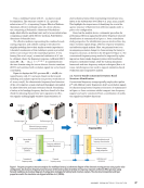
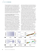
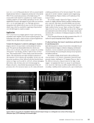
To visualize the frequency structure of both excitation and
reflection signals (s t ,r t ),we combine signal vectors with differ-
ent center frequencies into signal matrices (S t ,R t )in the time
domain and then generate their frequency-domain represen-
tations (S f ,R f )using the discrete Fourier transform (DFT). The
signal-based frequency response map can thus be formalized
as (Ren et al. 2025a Huang et al. 2022):
(3)
{
S f =DFT[s(1),⋯
t ,s
t
(N w )],|S f |=abs[Sf]
R f =DFT[rt1),⋯ (,r
t
(N w )]=DFT[st1),⋯ (,s
t
(N w )]⊙ h 0 ,|R f |=abs[Rf]
where
S f ∈ ℂ N w × N s ′ and R f ∈ ℂ N w × N s ′ are the frequency signal
matrices for excitations and reflections under multiple
center frequencies specified by W sweep ,
h 0 stands for the system response coefficient at the 0-th
interface, which is the first column of H in Equation 1, and
|S f |and |R f |are the frequency-domain magnitude maps of
the excitation and reflection signals.
This signal-based formulation is suitable for both simula-
tion and experimental studies.
2.3. Frequency-Modulated Excitations for Battery Band
Structure Identification
In addition to the conventional method, we propose
using frequency-modulated excitations to enhance the
efficiency of the frequency sweep process. These excitation
signals can exhibit broadband frequency characteristics
controlled by instantaneous frequency modulations within
the time-frequency plane (Yang et al. 2019) and have been
widely reported across various engineering sectors, including
system identification and nondestructive testing (Chen et al.
2019 Challinor and Cegla 2024 Tian et al. 2024).
Frequency-modulated excitations can have different for-
mulations depending on their modulation characteristics.
Linear frequency-modulated excitations, also known as linear
chirps, can be constructed by introducing a linear increment
in the instantaneous frequency (IF) of the oscillation signal in
Equation 2. The IF can be expressed as:
f inst =f 0 ∙ 1 +α ∙ t ∈ ℝ N s
where
f 0 is the initial frequency,
1 ={1}Ns1
i= represents the all-ones vector, and
α is the chirp rate.
The linear frequency-modulated excitation, therefore, has
the form:
(4) s t
(α,β) =w ⊙ sin{2π[(f0 ∙ 1) ⊙ t +α
2
∙ (t ⊙ t)]}
where
u1D6DF inst =2π[(f0 ∙ 1) ⊙ t +α
2
∙ (t ⊙ t)] is the instantaneous phase
of the signal, and
w denotes the amplitude modulation term of the signal.
For a basic linear chirp, we can specify the amplitude term
as:
(5) w =1 t≤β ={1 t i ≤β }i=1
N S =
{
1, t i ≤ β
0, t i β
where
β is a user-specified parameter controlling the time duration
of the signal.
Equation 5 indicates that no amplitude modulation is applied
to the chirp aside from the zero-padding associated with β .
Additionally, windowed signals can be used to alter
the amplitude patterns of the linear chirp in Equation 5. To
maintain consistency with the narrow-band tonebursts in
Equation 2, the amplitude modulator includes Gaussian and
Hanning components and can be expressed as:
(6) w =exp
[
− t ⊙ t _
2 (
β _
2 √
_2ln2) ]
⊙ 0.5
[
1 − cos
(
2πt
β )]
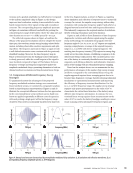
Note that modulated chirp excitations in Equation 6
employ different frequency sweep strategies compared to the
narrow-band tonebursts described in Section 2.2, due to their
distinct parameterizations of time-frequency behavior. Given
an initial frequency f 0 and a frequency bandwidth γ ,the fre-
quency range to be traversed is [f 0, f 0 +γ ].We can therefore
specify the time-frequency angle vector u1D6C9 =[θ 1 ,⋯ ,θ N θ ]T .
The waypoints within the parameter space spanned by
(u1D6C2,u1D6C3) of the chirp signals can then be derived as:
u1D6C2 =tan[u1D6C9]
ME
|
ELECTRICVEHICLES
48
M AT E R I A L S E V A L U AT I O N • J A N U A R Y 2 0 2 6

and
u1D6C3 =γ ⋅ u1D6C2 −1 ,
where
u1D6C2 −1 =[1/α1,1/α2, …]Tdenotes the element-wise inverse of
the chirp rate vector u1D6C2 .
Inspired by frequency response analysis techniques in
machining dynamics (Schmitz and Smith 2019 Ren and Ding
2022) and electrochemical impedance spectroscopy (EIS) (Yang
and Rogach 2019), we leverage these parametrized chirp signals to
probe the ultrasonic frequency response structure. By combining
response wave analytics with time-frequency spectra (Ren et al.
2025a Gröchenig 2001 Yang et al. 2019), the proposed excitation
strategy enables efficient characterization of the crucial band
structure over specified frequency ranges for multilayer batteries.
3. Results and Discussion
This section presents verification of the proposed method
through simulation-based case studies. The performance of
the linear frequency sweep and the angular frequency sweep is
comparatively investigated, highlighting the advantages of opti-
mizing excitation designs in high-throughput testing.
3.1. Verification of Linear Frequency Sweep Using
Single-Frequency Excitations
To assess the viability of using narrow-band, single-frequency
excitations for identifying battery frequency band struc-
tures, a series of linear frequency sweep simulations was
conducted. The sampling frequency was set to f s =500 MHz
with N s =5 × 10 4 sampling points. Toneburst signals with
a width of N c =5 cycles and center frequencies spanning
W sweep =[1.00, 1.01, ⋯ ,3.00] MHz were considered. The results
are presented in Figure 2.
As shown in Figure 2a, the magnitude map |S f |of the exci-
tation signals exhibits a clear diagonal pattern, reflecting the
alignment between the specified center frequencies and the
dominant signal frequencies. In contrast, the magnitude map
|R f |of the reflection signals in Figure 2c displays a local dis-
continuity with suppressed wave intensity. This corresponds
to the stopband behavior induced by the internal multilayer
architecture of the cell, indicating the presence of a frequency
bandgap that strongly attenuates reflected signal energy (Ren
et al. 2025a, 2025b).
To further examine the frequency-structure characteristics
under individual center frequencies, Figures 2b and 2d display
the time-frequency spectra of both excitation and reflection
signals for three representative excitation frequencies indicated
by ①–③. At 1.00 MHz, the reflection signal retains strong
energy and a compact waveform, indicating minimal distortion
induced by wave–battery interactions. At 1.95 MHz—situated
within the battery bandgap—the reflected waveform under-
goes significant distortion and splitting, suggesting destructive
interference and strong energy suppression (Huang et al. 2022
Ren et al. 2025a). At 2.75 MHz, the reflection signal recovers a
relatively compact shape but exhibits slight frequency shifts.
These findings confirm that the reflection waveforms reveal
frequency-selective propagation within the battery, allowing
the battery band structure to be identified through conven-
tional frequency sweep tests.
It should be noted that the narrow-band nature of
single-frequency excitations requires a step-by-step sweep across
a specified range of center frequencies, whether in simulations
or experiments. To achieve sufficient frequency resolution, the
Center frequency (MHz)
1
2
3
1 2 3
1
0 1
2 3
Center frequency (MHz)
1
2
3
1 2 3
1
0
4
5 6
Bandgap
0 5 10 15
TOF (μs)
3
2
1
0 5 10 15
TOF (μs)
3
2
1
0 5 10 15
TOF (μs)
3
2
1
1
0.25
4
5
6
1.95 MHz
2.75 MHz
1.00 MHz
0 5 10 15
TOF (μs)
3
2
1
0 5 10 15
TOF (μs)
3
2
1
0 5 10 15
TOF (μs)
3
2
1
1
0.25
1
2
3
1.95 MHz
2.75 MHz
1.00 MHz
Figure 2. Battery band structure characterized by conventional frequency sweep tests using single-frequency excitations: (a, c) frequency magnitude
maps of excitation and reflection signals (b, d) time-frequency intensity (TFI) diagrams under sparsely selected center frequencies (①–⑥).
J A N U A R Y 2 0 2 6 • M AT E R I A L S E V A L U AT I O N 49
Toneburst frequency
(MHz)
Response
signal
frequency
(MHz)
Center
frequency
(MHz)
Center
frequency
(MHz)
|S
f
|(a.u.)
|R
f
|(a.u.)
TFI (a.u.)
TFI (a.u.)