frequency step length may need to be reduced to the order of
10 −2 MHz, implying that more than 10 2 individual measure-
ments are needed to cover just a 1 MHz bandwidth (Ren et al.
2025a). In practice, such repeated tuning and acquisition can
significantly prolong testing time, increase instrument overhead,
and complicate signal stabilization, making single-frequency
sweeping inefficient for high-throughput ultrasonic battery
testing, particularly in manufacturing (McGovern et al. 2023).
This motivates the use of frequency-modulated excitations that
provide broader time-frequency coverage, thereby improving the
effectiveness of the traditional frequency sweep method.
3.2. Verification of Angular Frequency Sweep Using
Frequency-Modulated Excitations
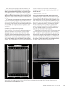
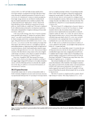
To address the inefficiencies of single-frequency sweep tests,
we investigate the use of frequency-modulated chirp exci-
tations for probing the frequency response structure of mul-
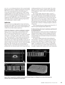
tilayer batteries. The excitation signal is designed using the
formulation in Equations 4 and 5, with a linear chirp rate
of α =0.1 MHz/µs, initial frequency f 0 =0.75 MHz, and time
duration β =20 µs. The resulting waveform spans a frequency
range of approximately [0.75, 2.75] MHz, consistent with the
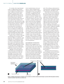
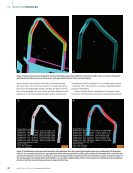
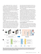
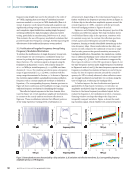
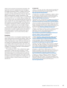
sweep range demonstrated in Section 3.1. As shown in Figure 3a,
the excitation signal exhibits a gradually increasing oscillation
frequency with a constant amplitude envelope as defined in
Equation 5. The corresponding frequency-domain spectrum in
Figure 3b shows continuous and broadband coverage, ensuring
sufficient frequency resolution for identifying the bandgap.
The reflected signal response in the time domain, illus-
trated in Figure 3d, reveals significant amplitude modulations,
in contrast to the nearly uniform toneburst reflections in
Figure 3a. These modulations indicate that different portions
of the chirp experience varying levels of attenuation or
enhancement, depending on the instantaneous frequency, as
further verified in the frequency spectrum shown in Figure 3e.
A distinct dip in the reflection amplitude appears around the
critical frequency of 2 MHz, consistent with the previously
observed bandgap position in Figures 1b and 2d.
Figures 3c and 3f display the time-frequency spectra of the
excitation and reflection signals. The chirp excitation shows
a well-defined linear ridge in the spectrum, consistent with
its constant sweep rate. In contrast, the reflection spectrum
reveals a pronounced disruption around the bandgap
frequency, forming a visually identifiable intensity gap in the
time-frequency ridge. These results indicate that chirp exci-
tations not only compress the traditional sweep into a single
shot but also preserve the spectral sensitivity necessary for
bandgap identification. Meanwhile, the simulations confirm
that no additional bandgap exists within the investigated fre-
quency range of [1, 3] MHz. This conclusion is supported by
three types of evidence: (1) the FRC spectrum in Figure 1b, (2)
the time-frequency spectra under single-frequency excitations
in Figures 2b and 2d, and (3) the time-frequency spectra under
frequency-modulated excitations in Figures 3c and 3f. In par-
ticular, the loss of response intensity around the critical fre-
quency of 2 MHz is clearly observed, where reflection waves
are strongly modulated and split into two sections along the
time-of-flight axis, evidencing the bandgap effect.
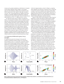
To further improve the time localization and practical
applicability of chirp-based excitations, we introduce an
amplitude-modulated chirp by applying a composite window
function to the linear frequency-modulated signal. As for-
mulated in Equation 6, the modulation involves a Gaussian–
Hanning window envelope that shapes the chirp into a
temporally compact waveform. Figure 4a shows the result-
ing excitation signal, which exhibits both a linear frequency
ME
|
ELECTRICVEHICLES
0 5 10 15 20
TOF (μs)
5
4
3
2
1
0
1
0.25
1
2
0 2.5 5
Frequency (MHz)
1
0
Bandgap
1 2
0 5 10 15 20
TOF (μs)
1
0
–1
Amplitude modulation
0 5 10 15 20
TOF (μs)
5
4
3
2
1
0
1
0.25
1
2
Bandgapgapdan B
Critical frequency
0 5 10 15 20
TOF (μs)
1
0
–1
0 2.5 5
Frequency (MHz)
1
0 1 2
2.75 MHz
0.75 MHz
Figure 3. Battery band structure characterized by a chirp excitation: (a, d) excitation and reflection waveforms (b, e) corresponding frequency
amplitude spectra (c, f) TFI diagrams.
50
M AT E R I A L S E V A L U AT I O N • J A N U A R Y 2 0 2 6
Frequency
(MHz)
Amplitude
(a.u.)
Amplitude
(a.u.)
Frequency
(MHz)
Amplitude
(a.u.)
Amplitude
(a.u.)
TFI (a.u.)
TFI (a.u.)

increase and a gradual amplitude rise–fall behavior. Compared
to the uniform-amplitude chirp in Figure 3a, this design
improves time localization, making it more suitable for echo-
based measurements where signal overlap and crosstalk are
concerns. The corresponding frequency-amplitude spectrum
in Figure 4b maintains sufficient bandwidth for probing the
critical frequency range of the battery, where the chirp rate and
time duration are set as α =0.1 MHz/µs and β =18.75 µs.
The reflected response shown in Figure 4d confirms the
efficacy of the proposed modulation scheme: despite the shorter
time span, the waveform retains strong bandgap-related defor-
mation, including observable wavefront suppression and split-
ting effects. The frequency spectrum in Figure 4e again reveals
a well-defined attenuation zone consistent with the previously
identified bandgap. Moreover, the time-frequency map in
Figure 4f demonstrates that the bandgap-induced disruption
is clearly preserved, while the overall footprint of the signal is
more localized compared to Figure 3f. This balance between
frequency coverage and temporal compactness makes the
amplitude-modulated chirp a promising alternative to both tra-
ditional toneburst excitations and long-duration linear chirps.
3.3. Comparison of Different Frequency Sweep
Strategies
To quantitatively assess the advantages of the proposed
frequency-modulated excitation strategy over conventional
linear toneburst sweeps, we conducted a comparative analysis
based on time-frequency representations. Figures 5a and 5b
illustrate the conceptual difference between the two approaches.
In the conventional linear sweep method, narrow-band tone-
bursts are applied sequentially at different center frequencies,
with each probing a single point within the frequency range
of interest. This creates a horizontally stacked sweep trajectory
in the time-frequency plane, as shown in Figure 5a, requiring
dense simulation and collection of response traces to ensure full
coverage. In contrast, the angular sweep strategy utilizes chirp
excitations with varying time-frequency angles θ and achieves a
diagonal traversal across both time and frequency dimensions.
This inherently compresses the required number of excitations,
thereby reducing redundancy and sweep duration.
Figures 5c and 5d offer a direct illustration of time-frequency
diagrams for excitation and reflection signals using the angular
sweep methodology. Six modulated chirp signals with time-
frequency angles θ =[70, 60, 50, 40, 30, 20]T degrees are employed,
ensuring comprehensive coverage of the targeted frequency
range [0.75, 2.75] MHz with diverse temporal supports. The
resulting time-frequency intensity (TFI) trajectories sweep diag-
onally across the entire domain, establishing a sequence of dis-
tributed and oblique ridge patterns. The crucial frequency struc-
ture of the battery is consistently identified across these angular
waypoints, each offering a distinctive and informative characteri-
zation of the bandgap with no redundant frequency sampling.
Based on the analysis above, we can summarize the key
performance advantages of the angular chirp sweep strategy
as follows. Compared to the conventional linear sweep, the
angular approach requires fewer sweeping points due to its
broader time-frequency coverage, thereby reducing redundant
simulations or experimental measurements and improving
the efficiency of frequency structure identification. For the
[0.75, 2.75] MHz frequency range, the angular sweep strategy
requires only sparse measurements on the order of 10 1 to
characterize the critical band structure of the battery using
different time-frequency information. In contrast, the con-
ventional linear sweep requires dense measurements on the
order of 10 2 to resolve the battery bandgap, resulting in unnec-
essary scanning of less informative frequency regions and
0 2.5 5
Frequency (MHz)
1
0
1 2
2.75 MHz
0.75 MHz
0 5 10 15 20
TOF (μs)
1
0
–1
0 5 10 15 20
TOF (μs)
1
0
–1 Wave modulation
0 2.5 5
Frequency (MHz)
1
0
Bandgap
1 2
0 5 10 15 20
TOF (μs)
5
4
3
2
1
0
1
0.25
1
2
0 5 10 15 20
TOF (μs)
5
4
3
2
1
0
1
0.25
1
2
Bandgapa
Critical frequency
B
Figure 4. Battery band structure characterized by an amplitude-modulated chirp excitation: (a, d) excitation and reflection waveforms (b, e)
corresponding frequency amplitude spectra (c, f) TFI diagrams.
J A N U A R Y 2 0 2 6 • M AT E R I A L S E V A L U AT I O N 51
Amplitude
(a.u.)
Amplitude
(a.u.)
Amplitude
(a.u.)
Amplitude
(a.u.)
Frequency
(MHz)
Frequency
(MHz)
TFI (a.u.)
TFI (a.u.)