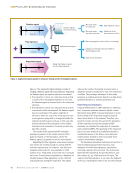
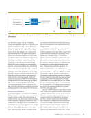
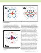
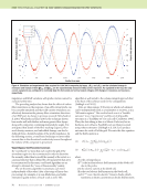
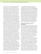
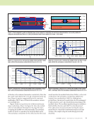
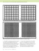
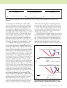
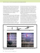
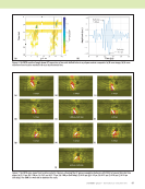
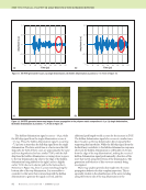
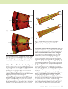
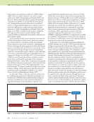
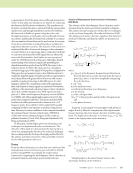
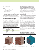
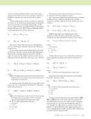
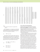
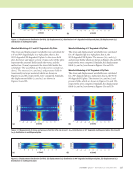
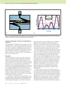
108 M A T E R I A L S E V A L U A T I O N • J A N U A R Y 2 0 2 0 (4) where spik is the stress tensor at y point due to the source at y0 with force acting along the p-th direction, Cikmj is the stiffness matrix, and epmj is the strain tensor. Please note that the distance vector in Equation 4 is x = y – y0. By looking at Equation 4, we can see that the Cijkl matrix is essential for modeling the ultrasonic field. First, we need to know if and how the Cijkl matrix is affected by the presence of microscale damages. Effect of Microscale Damage (Void) in the Cijkl Matrix To understand the effect of microscale damage such as voids on the effective material properties, a representative volume element (RVE) is developed. An RVE with length, width, and height of 62 μm is simulated to obtain the pristine constitutive coefficients using the finite element method (Swaminathan et al. 2006 Swaminathan and Ghosh 2006). The fiber diameter is 7 μm and the fiber volume fraction is 50%. Interfaces between the fiber and matrix were assumed to be perfectly bonded. The material properties of the fiber and the matrix are tabulated in Table 1. The RVE technique utilized by Swaminathan (Swaminathan et al. 2006 Swaminathan and Ghosh 2006) is employed to govern the size of a RVE with void contents, and the size of the RVE is calculated subsequently. The size of the RVE for UD composite with void contents was 90 μm. The RVE schematics with spherical and ellipsoid void contents and mesh generation for the RVEs are shown in Figure 2. The void measurements such as center and radius are randomly generated (Tavaf et al. 2018a, 2018b) by means of normal distribution. The void measure- ments are monitored such that the voids are not in interfer- ence with the fibers. The process is repeated until the desired configuration is acquired. A unit cell with different distributions of voids is simulated to understand the effect of various distributions on the effective material properties when the percentage of the void content is constant and the void shape is spherical. Data were generated through FEM simulation by applying periodic boundary conditions and error bounds were estimated within 3× the standard deviation, wings out from the mean value. The detailed technique is quite intensive and omitted herein due to limited space but can be found in other research (Tavaf et al. 2019). A similar study was conducted with an ellipsoid void shape. Thus, both spherical voids between randomly generated fiber locations and ellipsoid void shapes parallel to the fiber direction are modeled into the unit cell to thoroughly understand the effect of void shapes on constitu- tive coefficients. Next, the RVEs with different void contents were analyzed. The full matrix of effective material properties was found. The perturbation of each constitutive coefficient with respect to increasing the void percentage in the RVE is shown in Figure 3. The normal coefficients on the matrix of effective material property are decreased by increasing the void content as seen in Figure 3. C11 and C22 decreased by approximately 8%, and C33 decreased by approximately 12% with 5% void content. All the shear coefficients also degraded due to the C x x) p ik ikmj mj ( ) ( fi = °p ME TECHNICAL PAPER w computational nde for composites 2 2 3 3 1 1 90 μm 90 μm 90 μm 90 μm Figure 2. Schematic of a representative volume element for: (a) spherical voids (b) ellipsoid voids and (c) mesh generation (Zhao and Rose 2003). (a) (b) (c) TABLE 1 Material properties of fiber and matrix T 300 Carbon Fiber Epoxy 230 Efl (GPa) 5 E (GPa) 15 Efv (GPa) 0.16 v 0.25 vfl – 0.07 vfv – 90 μm 90 μm

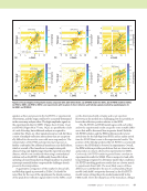
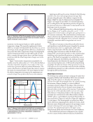
J A N U A R Y 2 0 2 0 • M A T E R I A L S E V A L U A T I O N 109 presence of voids. C31 and C32 decreased by approximately 10% and C21 decreased by approximately 4%. C31 and C32 have higher degradation compared to C21 since the matrix carries less stresses along the perpendicular to the fiber direc- tion compared to pristine state. C44, C55, and C66 decreased by almost 8%. However, the degradation of C66 is higher than C55 since the matrix contributes to carry the load. All percentages of degradation are calculated from the third-order polynomial trend line within the calculated error bound. The percentage of degradation of each element in the constitutive matrix due to 5% void is calculated (Tavaf et al. 2019) and is presented below: DPSM Formulation of the CNDE Problem In this section, the CNDE problem is introduced and the DPSM formulation is derived for the problem. The wavefield in the anisotropic multilayered plate is numerically computed after the DPSM formulation. DPSM Formulation in Anisotropic Multilayered Plate An NDE problem for a multilayered plate (shown in Figure 4a) is modeled using DPSM. A 3 mm thick multilayered (90/0)2 4-ply composite plate immersed in water is used to investigate using the traditional NDE mode. The plate is bound by two solid–fluid interfaces. Two ~1 MHz trans- ducers with a 2 mm diameter are placed symmetrically on either side of the plate in water at a 5 mm distance from the fluid–solid interface. To visualize the frequency domain wave phenomena inside anisotropic media, ultrasonic wavefields were simulated in transversely isotropic materials using their respective Green’s function. The DPSM technique is described based on the NDE problem being solved. DPSM, as the name suggests, is the technique based on distributing the source and target points in the actuator, such as the transducer and boundary and C5%void =# &8.8% &4.2% &10.1% 0 0 0 &4.2% &8.2% &10.1% 0 0 0 &10.1% &10.1% &11.9% 0 0 0 0 0 0 &8.5% 0 0 0 0 0 0 &8.3% 0 0 0 0 0 0 &8.8% % $ # # # # # # " ! 0 7.4 7.8 8.2 8.6 1 2 3 Void percentage 4 5 0 7.2 7.7 8.2 8.7 1 2 3 Void percentage 4 5 0 100 106 112 118 1 2 3 Void percentage 4 5 0 1.21 1.23 1.25 1.27 1 2 3 Void percentage 4 5 0 1.8 1.9 2.0 2.1 1 2 3 Void percentage 4 5 0 1.8 1.9 2.0 2.1 1 2 3 Void percentage 4 5 0 4.4 4.6 4.7 4.9 1 2 3 Void percentage 4 5 0 4.2 4.6 4.4 4.8 5.0 1 2 3 Void percentage 4 5 0 3.2 3.3 3.5 3.6 1 2 3 Void percentage 4 5 Figure 3. Perturbation to the constitutive coefficients due to the different percentage of void contents fitted by third-order polynomial bounded by error within 3σ: (a) C11 (b) C22 (c) C33 (d) C21 (e) C31 (f) C32 (g) C44 (h) C55 and (i) C66. Red dots show the mean values. (a) (b) (c) (d) (e) (f) (g) (h) (i) C11 (GPa) C22 (GPa) C33 (GPa) C21 (GPa) C31 (GPa) C32 (GPa) C44 (GPa) C55 (GPa) C66 (GPa)