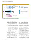
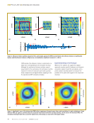
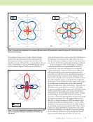
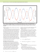
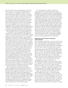
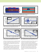
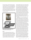
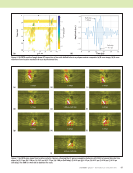
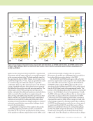
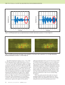
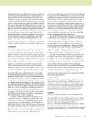
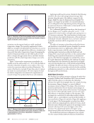
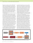
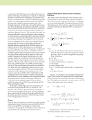
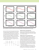
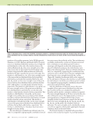
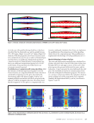
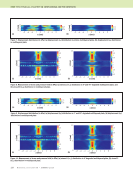
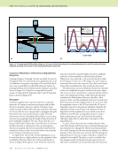
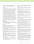
there are no fibers, and we must simply have resin. As far as eddy currents are concerned, the resin looks just like free space. Therefore, we conclude that as FAWT decreases, conductivity decreases toward zero (free space). If we take into account capacitive effects, we must look at the dielectric properties of the resin. Capacitive effects should not come into the picture for eddy current inspection, as long as we keep the frequencies relatively low. As FAWT increases, the prepreg begins to look more and more like a slab of solid carbon. An increasing number of fibers contact, making the transverse conductivity increase. It seems reasonable to assume that as FAWT increases, both the transverse and longitudinal conductivity approach a limit determined by the conductivity of the graphite fibers. We can probably improve somewhat on these simple-minded observations by using models for graphite fiber interactions found in the literature. We note that the transverse conductivity is likely to be more affected by a change in FAWT than the longitudinal conductivity, assuming a nominal value of 60% fiber. A simple argument is based on our previous comments. Assuming that the transverse conductivity, denoted sT , approaches the longitudinal conductivity, sL, as the fiber density approaches 100%, and given a typical anisotropy ratio of 200 to 1 (based on 60% fiber density), one can get an idea of how sT and sL must change when the fiber density is increased toward 100%. We note that sT must change by at least a factor of 200, while sL is known to change by only a factor of about two. Such a refined estimate of conductivity change will be useful when we assess the accuracy of the proposed method of measure- ment. For now, it will be reasonable to assume that the conductivity scales by the same percentage change as the FAWT (the transverse and longitudinal conductivities). Actually, it is suggested that the change in transverse conduc- tivity is a higher order than a direct-proportion relationship the simple model used by Treece et al. (1990) predicts a squared relationship. If indeed the transverse conductivity depends on the FAWT squared, or a higher power of FAWT, then we are in a good position to measure the FAWT change. We know from our own experience and models that eddy current measurements are sensitive to conductivity changes in carbon fiber composites. All that remains to be discovered is the relationship between conductivity and FAWT. Resin content appears to affect the conductivity in a perhaps complicated way. It appears that resin content can dramatically affect the transverse conductivity but may have little effect on the longitudinal conductivity. One way to explain the physical reason for the conductivity change with resin content is to think of the resin as an insulator partially shielding the adjacent fibers (“wires”) from contacting each other, thereby reducing sT. Using this explanation also leads us to the conclu- sion that sL is not significantly changed by resin content, assuming that the resin content does not significantly change the overall volume of the material, since the “wires” conduct equally well when they are surrounded by insulation. It is somewhat easier to predict the variation of a measured signal when the conductivity of the sample is changed than it is to predict the variation of the signal when the FAWT is changed. The problem is somewhat simplified if the sample thickness is known a priori, but knowledge of the sample thickness should not be a requirement. The collection of multifrequency data with a T/R array presumably could be used to independently extract FAWT and sample thickness, with the interrogating field distribution varied both by skin depth attenuation and T/R coil pair geometrical effects. The model is useful in generating the prediction of signal variation when the conductivity changes. Another possible technique, other than the computer model, for determining the relation- ship between conductivity and measured signal would be to measure the signal given known-conductivity samples. It is unlikely, however, that we would have enough samples to accurately determine the response to conductivity change using strictly experimental data. A useful approach might be to use the model in conjunction with experimental data to determine a better approximation of the relationship. Anisotropic Inverse Problem for Composite Characterization The model problem, adapted from a previous work (Fast et al. 2015), is shown in Figure 5. The test region is discretized into an 8 × 8 array in the plane of the sample surface with four layers in the z direction. Cells are labeled from zero beginning at the minimum coordinate for each dimension such that [k, l, m] = [0 : 7, 0 : 7, 0 : 3] in Equations 1 through 5. The conductivity parallel and transverse to the fiber directions are taken from Table 1. The crack region contained in the third layer (m = 2) is two cells wide and extends the full eight cells of the length of the test region. The anomalous conductivity is fixed to zero for the bottom layer (m = 0), which is host material. Note that the total conductivity of each cell is equal to the anomalous conductivity plus the host conductivity. We simulate a 41 × 41 receiving array and an 11 × 11 transmitting array, so that Ns = 1681 and u = 1, . . . , 121 in Equations 3 through 5. This means that there will be 121 “experiments” with 242 outcomes, the real and imaginary parts of (Ex, Jx) and (Ey, Jy) for the conductivity of each discretized cell. There are 8 × 7 × 3 unknown coefficients for Jx and 8 × 7 × 3 unknown coefficients for Jy, giving a total of 336 unknowns for the data equation. Thus, with 1681 equa- tions and 336 unknowns, the problem is highly overdetermined. Figures 6 to 9 show the inversion process for a cell near the middle of the top (klm = 333) and the cracked (klm = 332) layers. In these figures the dots are the “experi- mental outcomes,” the real and imaginary parts of (Ex, Jx) and (Ey, Jy) induced by each of the 121 transmitter coils. Each of these 242 outcomes is calculated from Equations 3 and 5 and incorporates the response of all 1681 receiver coils. The best linear fit to the current versus field plots is then obtained using the least-median-of-squares robust estimator. The slope 78 M A T E R I A L S E V A L U A T I O N • J A N U A R Y 2 0 2 0 ME TECHNICAL PAPER w eddy current characterization for cfrp composites

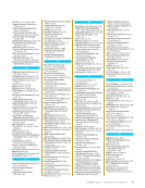
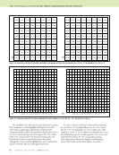
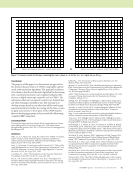
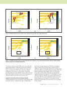
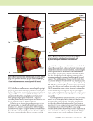
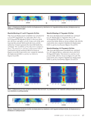
J A N U A R Y 2 0 2 0 • M A T E R I A L S E V A L U A T I O N 79 of this line is the estimated anomalous conductivity. Note that the scatter in the data for the cross-ply conductivity in the top layer, Figure 8, appears exaggerated due to the extremely small range of the Y axis, as all inverted anomalous currents are essentially zero. Figure 10 shows a top-down view of the inverted anom- alous conductivity of layer 2 in Figure 5b. Here, the cracked cells run vertically from the bottom to the top of the layer, occupying the middle two cells horizontally. The inversion results are shown to reproduce the model problem nicely. The anomalous conductivity for the cells away from the crack exactly matches the modeled values from Table 1, as the total conductivity is the anomalous conductivity added to the isotropic host conductivity of 100 S/m. Although not pictured here, the inverted conductivities for the undamaged 0° plies in layers 1 and 3 also found identical matching to the modeled values. The excellent reproduction gives confidence that both fiber direction and FAWT can be determined from eddy current measurements by inverting the experi- mental data to a discretized conductivity tensor across the volume of the sample using the methodology previously described. 0° 90° 0° 0 mm 0.1 mm 0.2 mm 0.3 mm 0.4 mm Crack σ x = σ y = σ z = 100 500 μm 0° 90° 0° 100– 200 μm Figure 5. Electromagnetic model and detailed view of test region for composite microstructure characterization: (a) model problem for composite microstructure (Fast et al. 2015) (b) detailed view of test region (152.4 mm × 152.4 mm). (a) (b) –1.2×106 –1×106 –800 000 –600 000 –400 000 –200 000 0 200 000 400 000 600 000 800 000 1×106 –60 –50 –40 –30 –20 –10 0 10 20 30 40 50 E x Real Imaginary J x = 19 900*E x Figure 6. Jx versus Ex for a cell near the middle of the top (klm = 333) layer, where the anomalous conductivity for (k,l,m) = (3, 3, 3). –200 000 –150 000 –100 000 –50 000 50 000 100 000 –1000 –500 0 0 500 1000 1500 2000 E x Real Imaginary J x = –85.25*E x Figure 7. Jx versus Ex for a cell near the middle of the cracked (klm = 332) layer, where the anomalous conductivity for (k,l,m) = (3, 3, 2). –4000 –3×10–8 –4×10–8 –2×10–8 –1×10–8 0 1×10–8 2×10–8 3×10–8 4×10–8 –2000 0 2000 4000 6000 8000 10 000 E y Real Imaginary J y = 6.670E-13*E y Figure 8. Jy versus Ey for a cell near the middle of the top (klm = 333) layer, where the anomalous conductivity for (k,l,m) = (3, 3, 3). –150 000 –100 000 –50 000 0 50 000 100 000 150 000 200 000 250 000 300 000 –3000 –2000 –1000 0 1000 E y Real Imaginary J y = –100*E y Figure 9. Showing Jy versus Ey for a cell near the middle of the cracked (klm = 332) layer, where the anomalous conductivity for (k,l,m) = (3, 3, 2). J x J x J y J y